Can the Exadata Smart Flash Cache slow smart scans?

I’ve been doing some work on the Exadata Smart Flash Cache recently and came across a situation in which setting CELL_FLASH_CACHE to KEEP will significantly slow down smart scans on a table.

If we create a table with default settings, then the Exadata Smart Flash Cache (ESFC) will not be involved in smart scans, since by default only small IOs get cached.  If we want the ESFC to be involved, we need to set the CELL_FLASH_CACHE to KEEP.  Of course, we don’t expect immediate improvements, since we expect that the next smart scan will need to populate the cache before subsequent scans can benefit. 

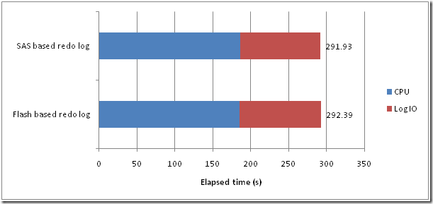
HOWEVER, what I’m seeing in practice is that the next smart scan following an ALTER TABLE … STORAGE(CELL_FLASH_CACHE KEEP) is significantly degraded, while subsequent scans get a performance boost.  Here’s an example of what I observe:

image


The big increase in CELL IO time is in an increase in both the number and latency of cell smart table scans.  The wait stats for the first scan with a default setting looked like this:

Elapsed times include waiting on following events:
  Event waited on                             Times   Max. Wait  Total Waited
  ----------------------------------------   Waited  ----------  ------------
  gc cr disk read                                 1        0.00          0.00
  cell single block physical read                 2        0.01          0.01
  row cache lock                                  2        0.00          0.00
  gc cr grant 2-way                               1        0.00          0.00
  SQL*Net message to client                    1021        0.00          0.00
  reliable message                                1        0.00          0.00
  enq: KO - fast object checkpoint                2        0.00          0.00
  cell smart table scan                        9322        0.14          7.60
  SQL*Net message from client                  1021        0.00          0.02

For the first scan with KEEP cache it looked like this:

Elapsed times include waiting on following events:
  Event waited on                             Times   Max. Wait  Total Waited
  ----------------------------------------   Waited  ----------  ------------
  SQL*Net message to client                    1021        0.00          0.00
  reliable message                                1        0.00          0.00
  enq: KO - fast object checkpoint                2        0.00          0.00
  cell smart table scan                       14904        1.21         33.37
  SQL*Net message from client                  1021        0.00          0.02

Looking at the raw trace file didn’t help – it just shows a bunch of lines like this, with only a small number (3 in this case) of unique cellhash values… I couldn’t see a pattern:

WAIT #… : nam='cell smart table scan' ela= 678 cellhash#=398250101 p2=0 p3=0 obj#=139207 tim= …

I’m at a loss to understand why there would be such a high penalty for the initial smart scan with CELL_FLASH_CACHE KEEP setting.  You expect some overhead from constructing and storing the result set blocks in the cache, but an IO penalty of 200=300% seems way too high.   Anybody seen anything like this or have a clear explanation?

Test script is here, and formatted tkprof here

Redo on SSD: effect of redo size (Exadata)

Of all the claims I make about SSD for Oracle databases, the one that generates the most debate is that placing redo logs on SSD is not likely to be effective.  I’ve published data to that effect in particular see  Using SSD for redo on Exadata - pt 2 and 04 Evaluating the options for Exploiting SSD.

I get a lot of push back on these findings – often on theoretical grounds from Flash vendors (“our SSD use advanced caching and garbage collection that support high rates of sequential IO”) or from people who say that they’ve used flash for redo and it “worked fine”.

Unfortunately, every single test I do comparing performance of redo on flash and HDD shows redo with little or no advantage and in some cases with a clear disadvantage.    

One argument for flash SSD that I’ve heard is that while for the small transactions I use for testing  flash might not have the advantage but for “big” redo writes – such as those associated with LOB updates – flash SSD would work better.  The idea is that the overhead of garbage collection and free page pool processing is less with big writes since you don’t hit the same flash SSD pages in rapid succession as you would with smaller writes.    On the other hand a reader who knows more about flash than I do (flashdba.com) recently commented:  “in foreground garbage collection a larger write will require more pages to be erased, so actually will suffer from even more performance issues.”

It’s taken me a while to get around to testing this, but I tried on our Exadata X-2 recently with a test that generates a variable amount of redo and then commits.  The relationship between the size of the redo and redo log sync time is shown below

image


I’m now putting on my flame retardant underwear in anticipation of some dispute over this data….   but,  this suggests that while SSD and HDD (at least on Exadata) are about at parity for small writes, flash degrades much more steeply than HDD as the size of the redo entry increases.  Regardless of whether the redo is on flash or HDD, there’s a break at the 1MB point which corresponds to log buffer flush threshold.  When a redo entry is only slightly bigger than 1MB then the chances are high that some of  it will have been flushed already – see Redo log sync time vs redo size for a discussion of this phenomenon.

The SSD redo files were on an ASM disk group carved out of the Exadata flash disks - see Configuring Exadata flash as grid disk to see how I created these.  Also the redo logs were created with 4K blocksize as outlined in Using SSD for redo on Exadata - pt 2.   The database was in NoarchiveLog mode.  Smart flash logging was disabled.  As far as I can determine, there was no other significant activity on the flash disks (the grid disks were supporting all the database tablespaces, so if anything the SSD had the advantage). 

Why are we seeing such a sharp dropoff in performance for the SSD as the redo write increases in size?   Well one explanation was given by  flashdba in this comment thread.  It has to do with understanding what happens when a write IO which modifies an existing block hits a flash SSD.   I tried to communicate my limited understanding of this process in Fundamentals of Flash SSD Technology.   Instead of erasing the existing page, the flash controller will pull a page off a “free list” of pages and mark the old page as invalid.   Later on, the garbage collection routines will reorganize the data and free up invalid pages.  In this case, it’s possible that no free blocks were available because garbage collection fell behind during the write intensive workload.  The more blocks written by LGWR, the more SSD pages had to be erased during these un-optimized writes and therefore the larger the redo log write the worse the performance of the SSD.

Any other theories and/or observations?  

I hope soon to have a Dell system with Dell express flash so as I can repeat these tests on a non-exadata system.  The F20 cards used in my X-2 are not state of the art, so it’s possible that different results could be obtained with a more recent flash card, or with a less contrived workload.

However, yet again I’m gathering data that suggests that using flash for redo logs is not worthwhile.  I’d love to argue the point but even better than argument would be some hard data in either direction….

Exadata Write-back cache and free buffer waits

Prior to storage server software version 11.2.3.2.0 (associated with Exadata X3), Exadata Smart Flash Cache was a “write-through” cache, meaning that write operations are applied both to the cache and to the underlying disk devices, but are not signalled as complete until the IO to the disk has completed.

Starting with 11.2.3.2.0 of the Exadata storage software[1], Exadata Smart Flash Cache may act as a write-back cache. This means that a write operation is made to the cache initially and de-staged to grid disks at a later time. This can be effective in improving the performance of an Exadata system that is subject to IO write bottlenecks on the Oracle datafiles.

Writes to datafile generally happen as a background task in Oracle, and most of the time we don’t actually “wait” on these IOs. That being the case, what advantage can we expect if these writes are optimized? To understand the possible advantages of the write-back cache let’s review the nature of datafile write IO in Oracle and the symptoms that occur when write IO becomes the bottleneck.

When a block in the buffer cache is modified, it is the responsibility of the database writer (DBWR) to write these “dirty” blocks to disk. The DBWR does this continuously and uses asynchronous IO processing, so generally sessions do not have to wait for the IO to occur – the only time sessions wait directly on write IO is when a redo log sync occurs following a COMMIT.

However, should all the buffers in the buffer cache become dirty then a session may wait when it wants to bring a block into the cache – resulting in a “free buffer wait”.

image

Free buffer waits can occur in update-intensive workloads when the IO bandwidth of the Oracle sessions reading into the cache exceeds the IO bandwidth of the database writer. Because the database writer uses asynchronous parallelized write IO, and because all processes concerned are accessing the same files, free buffer waits usually happen when the IO subsystem can service reads faster than it can service writes.

There exists just such an imbalance between reads and write latency in Exadata X2 – the Exadata Smart Flash Cache accelerates reads by a factor of perhaps 4-10 times, while offering no comparable advantage for writes. As a result, a very busy Exadata X2 system could become bottlenecked on free buffer waits. The Exadata Smart Flash Cache write-back cache provides acceleration to datafile writes as well as reads and therefore reduces the chance of free buffer wait bottlenecks.

The figure below  illustrates the effectiveness of the write-back cache for workloads that encounter free buffer waits. The workload used to generate this data was heavily write-intensive with very little read IO overhead (all the necessary read data was in cache). As a result, it experienced a very high degree of free buffer waits and some associated buffer busy waits. Enabling the write-back cache completely eliminated the free buffer waits by effectively accelerating the write IO bandwidth of the database writer. As a result, throughput increased four fold.

image

However, don’t be misled into thinking that the write-back cache will be a silver bullet for any workload.  Workloads that are experiencing free buffer waits are likely to see this sort of performance gain. Workloads where the dominant waits are for CPU, read IO, global cache co-ordination, log writes and so on will be unlikely to see any substantial benefit from the write-back cache.   


[1] 11.2.3.2.1 is recommended as the minimum version for this feature as it contains fixes to significant issues discovered in the initial release.

Redo log sync time vs redo size

It’s been tough to find time to do actual performance research of late, but I have managed to get a test system prepared that will allow me to determine if Solid State disks offer some performance advantage over spinning disks when the redo entries are very large.   This is to test the theory that the results I’ve published in the past (here and here for instance) actually apply only when the redo entries are relatively small.  For small sequential writes to SSD, each successive write will invoke an erase of a complete NAND page, whereas in a larger sequential write  this will not occur since each write will hit different pages.

I’m still setting up the test environment to look at this, but first I thought it would be worth showing this pretty picture:

16-09-2013 9-08-26 PM redo sync2

This chart shows how redo log sync time (eg, time taken to COMMIT) varies with the amount of redo information written since the last COMMIT.  There is a slight overall upwards trend, but the really noticeable trend is the “sawtooth” effect, which I’ve highlighted below:

image

Can you guess what causes this?  

I think it’s pretty clear that we are seeing the effect of redo buffer flushing.  Remember, when you write redo entries, they are written to the redo buffer (or sometimes a strand).  Oracle flushes the buffer when you commit, but also flushes it when it is 1/3rd full, after 3 seconds (I think from memory) or after 1MB of redo entries.   Given that, we can see what happens when we commit:

  • If there has been no redo log flush since we started writing, we have to wait while LGWR writes all the entries to disk
  • If a redo log flush occurs after we have written our entries but before we COMMIT, then we have to write virtually nothing (but a COMMIT marker I suppose)
  • Between the two scenarios, we may have to write some of our redo log entries.  However, we should never have to write more than about 1MB

In the chart above we can clearly see the redo log flushes occurring at 1MB intervals.  If we write less than 1MB we generally have to write it all, above 1MB we only have to write a portion of the redo entry.     Note that on this system, I was pretty much the only session doing significant activity, so the pattern is very clear.  On a busy system the effect would be randomized by others causing flushes to occur.

Hopefully I’ll soon be able to compare HDD and SSD performance to see if there are any significant differneces to these trends – the above data was generated by redo on SSD.

Using GET DIAGNOSTICS in MySQL 5.6

When Steven and I wrote MySQL Stored Procedure programming our biggest reservation about the new stored procedure language was the lack of support for proper error handling.  The lack of the SIGNAL and RESIGNAL clauses prevented a programmer from raising an error that could be propagated throughout a call stack properly, and the lack of a general purpose exception handler which could examine error codes at run time led to awkward exception handling code at best, and poorly implemented error handling at worst.

In 5.4 MySQL implemented the SIGNAL and RESIGNAL clauses (see http://guyharrison.squarespace.com/blog/2009/7/13/signal-and-resignal-in-mysql-54-and-60.html), which corrected half of the problem.  Now finally, MySQL 5.6 implements the ANSI GET DIAGNOSTICS clause and we can write a general catch-all exception handler.

Here’s an example:

image

The exception handler is on lines 10-27.  It catches any SQL exception, then uses the GET DIAGNOSTICS clause to fetch the SQLstate, MySQL error code and messages to local variables.  We then decide what to do for anticipated errors – duplicate or badly formed product codes and SIGNAL a more more meaningful application error.  Unexpected errors are RESIGNALed on line 24.

This is a great step forward for MySQL stored procedures – the lack of a means to programmatically examine error codes made proper error handling difficult or impossible.  This is a major step forward in maturity. 

Thanks to Ernst Bonat of www.evisualwww.com for helping me work through the usage of GET DIAGNOSTICS.

Exadata Smart Flash Logging–Outliers

In my last post, I looked at the effect of the Exadata smart flash logging.  Overall,  there seemed to be a slight negative effect on median redo log sync times.  This chart (slightly different from the last post because of different load and configuration of the system), shows how there’s a “hump” of redo log syncs that take slightly longer when the flash logging is enabled:

image

But of course, the flash logging feature was designed to improve performance not of the “average” redo log sync, but of the “outliers”. 

In my tests, I had 40 concurrent processes writing redo as fast as they could.  Occasionally this would result in some really long wait times.  For instance, in this trace you see an outlier of 291,780 microseconds (the biggest outlier in my tests BTW) within an otherwise unremarkable set of waits:

WAIT #47124064145648: nam='log file sync' ela= 1043 buffer#=101808 sync scn=1266588527 p3=0 obj#=-1 tim=1347583167588250
WAIT #47124064145648: nam='log file sync' ela= 2394 buffer#=130714 sync scn=1266588560 p3=0 obj#=-1 tim=1347583167590888
WAIT #47124064145648: nam='log file sync' ela= 932 buffer#=101989 sync scn=1266588598 p3=0 obj#=-1 tim=1347583167592057
WAIT #47124064145648: nam='log file sync' ela= 291780 buffer#=102074 sync scn=1266588637 p3=0 obj#=-1 tim=1347583167884090
WAIT #47124064145648: nam='log file sync' ela= 671 buffer#=102196 sync scn=1266588697 p3=0 obj#=-1 tim=1347583167885294
WAIT #47124064145648: nam='log file sync' ela= 957 buffer#=102294 sync scn=1266588730 p3=0 obj#=-1 tim=1347583167886575

To see if the flash logging feature was successful in removing these outliers, I extracted the top 10,000 waits from each of the roughly 8,000,000 waits I recorded in each category.  Here’s a plot (non-logarithmic) of those waits:

image

So – the flash log feature was effective in eliminating or at least reducing very extreme outlying redo log sync times.    Most redo log sync operations will experience no improvement or maybe even a slight degradation. But for the small number of log syncs that would have experienced a really excessive delay, the feature works as advertised – it reduces the chance of really excessive log file syncs. 

In my opinion, this effect doesn't imply that the flash can process a redo log write faster than the magnetic disks - in fact probably the opposite is true.  But given two desitinations to choose from, we avoid really long delays that occur when one of the destinations only is overloaded. 

Exadata smart flash logging

Exadata storage software 11.2.2.4 introduced the Smart flash logging feature.  The intent of this is to reduce overall redo log sync times - especially outliers - by allowing the exadata flash storage to serve as a secondary destination for redo log writes.  During a redo log sync, Oracle will write to the disk and flash simultaneously and allow the redo log sync operation to complete when the first device completes. 

Jason Arneil reports some initial observations here, and Luis Moreno Campos summarized it here.

I’ve reported in the past on using SSD for redo including on Exadata and generally I’ve found that SSD is a poor fit for redo log style sequential write IO.  But this architecture should at least do now harm and on the assumption that the SSD will at least occasionally complete faster than a spinning disk I tried it out. 

My approach involved the same workload I’ve used in similar tests.  I ran 20 concurrent processes each of which performed 200,000 updates and commits – a total of 4,000,000 redo log sync operations.  I captured every redo log sync wait from 10046 traces and loaded them in R for analysis.

I turned flash logging on or off by using an ALTER IORMPLAN command like this (my DB is called SPOT):

ALTER IORMPLAN dbplan=((name='SPOT', flashLog=$1),(name=other,flashlog=on))'

And I ran “list metriccurrent where objectType='FLASHLOG'” before and after each run so I could be sure that flash logging was on or off.

When flash logging was on, I saw data like this:

Before:

     FL_DISK_FIRST                     FLASHLOG     32,669,310 IO requests
     FL_FLASH_FIRST                    FLASHLOG     7,318,741 IO requests
     FL_PREVENTED_OUTLIERS             FLASHLOG     774,146 IO requests

After:

      FL_DISK_FIRST                     FLASHLOG     33,201,462 IO requests
     FL_FLASH_FIRST                    FLASHLOG     7,337,931 IO requests
     FL_PREVENTED_OUTLIERS             FLASHLOG     774,146 IO requests


So for this particular cell the flash disk “won” only 3.8% of times (7,337,931-7,318,741)*100/(7,337,931-7,318,741+33,201,462-32,669,310) and prevented no “outliers”.  Outliers are defined as being redo log syncs that would have taken longer than 500 ms to complete. 

Looking at my 4 million redo log sync times,  I saw that the average and median times where statistically significantly higher when the smart flash logging was involved:

> summary(flashon.data$synctime_us) #Smart flash logging ON
   Min. 1st Qu.  Median    Mean 3rd Qu.    Max.
    1.0   452.0   500.0   542.4   567.0  3999.0
> summary(flashoff.data$synctime_us) #Smart flash logging OFF
   Min. 1st Qu.  Median    Mean 3rd Qu.    Max.
   29.0   435.0   481.0   508.7   535.0  3998.0
> t.test(flashon.data$synctime_us,flashoff.data$synctime_us,paired=FALSE)

    Welch Two Sample t-test

data:  flashon.data$synctime_us and flashoff.data$synctime_us
t = 263.2139, df = 7977922, p-value < 2.2e-16
alternative hypothesis: true difference in means is not equal to 0
95 percent confidence interval:
33.43124 33.93285
sample estimates:
mean of x mean of y
542.3583  508.6763

Plotting the distribution of redo log sync times we can pretty easily see that there’s actually a small “hump” in times when flash logging is on (note logarithmic scale):

image

This is of course the exact opposite of what we expect, and I checked my data very carefully to make sure that I had not somehow switched samples.  And I repeated the test many times and always saw the same pattern.  

It may be that there is a slight overhead to running the race between disk and flash, and that that overhead makes redo log sync times slightly higher.  That overhead may become more negligible on a busy system.  But for now I personally can’t confirm that smart flash logging provides the intended optimization and in fact I observed a small but statistically significant and noticeable degradation in redo log sync times when it is enabled.

Getting started with Apache Pig

If, like me, you want to play around with data in a Hadoop cluster without having to write hundreds or thousands of lines of Java MapReduce code, you most likely will use either Hive (using the  Hive Query Language HQL) or Pig.

Hive is a SQL-like language which compiles to Java map-reduce code, while Pig is a data flow language which allows you to specify your map-reduce data pipelines using high level abstractions. 

The way I like to think of it is that writing Java MapReduce is like programming in assembler:  you need to manually construct every low level operation you want to perform.  Hive allows people familiar with SQL to extract data from Hadoop with ease and – like SQL – you specify the data you want without having to worry too much about the way in which it is retrieved.  Writing a Pig script is like writing a SQL execution plan:  you specify the exact sequence of operations you want to undertake when retrieving the data.  Pig also allows you to specify more complex data flows than is possible using HQL alone.

As a crusty old RDBMS guy, I at first thought that Hive and HQL was the most attractive solution and I still think Hive is critical to enterprise adoption of Hadoop since it opens up Hadoop to the world of enterprise Business Intelligence.  But Pig really appeals to me as someone who has spent so much time tuning SQL.  The Hive optimizer is currently at the level of early rule-based RDBMS optimizers from the early 90s.  It will get better and get better quickly, but given the massive size of most Hadoop clusters, the cost of a poorly optimized HQL statement is really high.  Explicitly specifying the execution plan in Pig arguably gives the programmer more control and lessens the likelihood of the “HQL statement from Hell” brining a cluster to it’s knees.

So I’ve started learning Pig, using the familiar (to me) Oracle sample schema which I downloaded using SQOOP.   (Hint:  Pig likes tab separated  files, so use the --fields-terminated-by '\t' flag in your SQOOP job). 

Here’s a diagram I created showing how some of the more familiar HQL idioms are implemented in Pig:

Note how using Pig we explicitly control the execution plan:  In HQL it’s up to the optimizer whether tables are joined before or after the “country_region=’Asia’” filter is applied.  In Pig I explicitly execute the filter before the join.    It turns out that the Hive optimizer does the same thing, but for complex data flows being able to explicitly control the sequence of events can be an advantage. 

Pig is only a little more wordy than HQL and while I definitely like the familiar syntax of HQL I really like the additional control of Pig.

Using SSD for redo on Exadata - pt 2

In my previous post on this topic, I presented data showing that redo logs placed on an ASM diskgroup created from exadata griddisks created from flash performed far worse than redo logs placed on ASM created from spinning SAS disks.

Of course, theory predicts that flash will not outperform spinning magnetic disk for the sequential write IOs experienced by redo logs, but on Exadata, flash disk performed much worse than seemed reasonable and worse than experience on regular Oracle with FusionIO SSD would predict (see this post).

Greg Rahn and Kevin Closson were both kind enough to help explain this phenomenon.  In particular, they pointed out that the flash cards might be performing poorly because of the default 512 byte redo block size and that I should try a 4K blocksize.   Unfortunately, at least on my patch level (11.2.2.3.2), there appears to be a problem with setting a 4K blocksize

ALTER DATABASE add logfile thread 1 group 9 ('+DATA_SSD') size 4096M blocksize 4096
*
ERROR at line 1:
ORA-01378: The logical block size (4096) of file +DATA_SSD is not compatible with the disk sector size (media sector size is 512 and host sector size is 512)

According to Greg, the F20 SSD cards are incorrectly reporting their physical characteristics and this is fixed in the current patch level.   Luckily, you can override the check by setting

ALTER SYSTEM SET "_disk_sector_size_override"=TRUE SCOPE=BOTH;

Greg and Kevin really know their stuff:  setting a 4k redo log block size resulted in dramatic improvements to redo log throughput – elapsed time reduced by 70%:

image

As expected,  redo log performance for SSD still slightly lags that of SAS spinning disks.     It’s clear that you can’t expect a performance improvement by placing redo on SSD, but at least the 4K blocksize fix makes the response time comparable.  Of course, with the price of SSD being what it is, and the far higher benefits provided for other workloads – especially random reads – it’s hard to see an economic rationale for SSD-based redo.    But at least with a 4K blocksize it’s tolerable.

When our Exadata system is updated to the latest storage cell software, I’ll try comparing workloads with the Exadata smart flash logging feature.

Amazon Elastic Map Reduce (EMR), Hive, and TOAD

Since my first post on connecting to Amazon Elastic Map Reduce with TOAD, we’ve added quite a few features to our Hadoop support in general and our EMR support specifically, so I thought I’d summarize those features in this blog post

Amazon Elastic Map Reduce is a cloud-based version of Hadoop hosted on Amazon Elastic Compute Cloud (EC2) instance.  Using EMR, you can quickly establish a cloud based Hadoop cluster to perform map reduce work flows. 

EMR support Hive of course, and Toad for Cloud Databases (TCD)  includes Hive support, so let’s look at using that to query EMR data.

Using the Toad direct Hive client


TCD direct Hive connection support is the quickest way to establish a connection to Hive.  It uses a bundled JDBC driver to establish the connection.

Below we create a new connection to a Hive server running on EMR:

image

  1. Right click on Hive connections and choose “Connect to Hive” to create a new Hive connection.
  2. The host address is the “Master” EC2 instance for your EMR cluster.  You’ll find that on the EMR Job flow management page within your Amazon AWS console.  The Hive 0.5 server is running on port 10000 by default.
  3. Specifying a job tracker port allows us to track the execution of our Hive jobs in EMR.  The standard Hadoop jobtracker port is 50030, but in EMR it’s 9600.
  4. It’s possible to open up port 10000 so you can directly connect with Hive clients, but it’s a bad idea usually.  Hive has negligible built-in security, so you’d be exposing your Hive data.   For that reason we support a SSH mode in which you can tunnel through to your hadoop server using the keypair file that you used to start the EMR job flow.  The key name is also shown in the EMR console page, though obviously you’ll need to have an actual keypair file.

The direct Hive client allows you to execute any legal Hive QL commands.  In the example below, we create a new Hive table based on data held in an S3 bucket (The data is some UN data on homicide rates I uploaded).

SNAGHTML9c66e8d

Connecting Hive to the Toad data hub


It’s great to be able to use Hive to exploit Map Reduce using familiar (to me) SQL-like syntax.  But the real advantage of TCD for Hive is that we link to data that might be held in other sources – like Oracle, Cassandra, SQL Server, MongoDB, etc.

Setting up a hub connection to EMR hive is very similar to setting up a direct connection.  Of course you need a data hub installed (see here for instructions), then right click on the hub node and select “map data source”:

Now that the hub knows about the EMR hive connection, we can issue queries that access Hive and – in the same SQL – other datasources. For instance, here’s a query that joins homicide data in Hive Elastic Map Reduce with population data stored in a Oracle database (running as Amazonn RDS:  Relational Database Service).  We can do these cross platform joins across a lot of different types of database sources, including any ODBC compliant databases, any Apache Hbase or Hive connections, Cassandra, MongoDB, SimpleDB, Azure table services:

In the version that we are just about to release, queries can be saved as views or snapshots, allowing easier access from external tools of for users who aren’t familiar with SQL.   In the example above, I’m saving my query as a view.


Using other hub-enabled clients


TCD isn’t the only product that can issue hub queries.  In beta today, the Quest Business Intelligence Studio can attach to the data hub, and allows you to graphically explore you data using drag and drop, click and drilldown paradigms:

It’s great to be living in Australia – one of the lowest homicide rates!

If you’re a hard core data scientist, you can even attach R through to the hub via the RODBC interface.  So for instance, in the screen shot below, I’m using R to investigate the correlation  between population density and homicide rate.  The data comes from Hive (EMR) and Oracle (RDS),  is joined in the hub, saved as a snapshot and then feed into R for analysis.  Pretty cool for a crusty old stats guy like me (My very first computer program was written in 1979 on SPSS).

image

Using flash disk for Redo on Exadata

In this Quest white paper and on my SSD blog here,  I report on how using a FusionIO flash SSD compares with SAS disk for various configurations – datafile, flash cache, temp tablespace and redo log.  Of all the options I found that using flash for redo was the least suitable, with virtually no performance benefit:

image

That being the case,  I was surprised to see that Oracle had decided to place Redo logs on flash disk within the database appliance, and also that the latest release of the exadata storage cell software used flash disk to cache redo log writes (Greg Rahn explains it here).   I asked around at OOW hoping someone could explain the thinking behind this, but generally I got very little insight.

I thought I better repeat my comparisons between spinning and solid state disk on our Exadata system here at Quest.  Maybe the “super capacitor” backed 64M DRAM on each flash chip would provide enough buffering to improve performance.  Or maybe I was just completely wrong in my previous tests (though I REALLY don’t think so :-/).

Our Exadata 1/4 rack has a 237GB disk group constructed on top of storage cell flash disk.  I described how that is created in this post.   I chose 96GB per storage cell in order to allow the software to isolate the grid disks created on flash to 4 24GB FMODs (each cell has 16 FMODs).    Our Exadata system has fast SAS spinning disks – 12 per storage cell for a total of 36 disks.  Both the SAS and SSD disk groups had normal redundancy.

I ran an identical redo-intensive workload on the system using SAS or SSD diskgroups for the redo logs.  Redo logs were 3 groups of 4GB per instance.   I ran the workload on it’s own, and as10 separate concurrent sessions.  

The results shocked me:

image

When running at a single level of concurrency,  the SSD based ASM redo seemed to be around 4 times slower than the default SAS-based ASM redo.  Things got substantially worse as I upped the level of concurrency with SSD being almost 20 times slower.  Wow.

I had expected the SAS based redo to win – the SAS ASM disk group has 36 spindles to write to, while the SSD group is (probably) only writing to 12 FMODs.  And we know that we don’t expect flash to be as good as SAS disks for sequential writes.  But still, the performance delta is remarkable. 

Conclusion


I’m yet to see any evidence that putting redo logs on SSD is a good idea, and I keep observing data from my own tests indicating that it is neutral at best and A Very Bad Idea at worse.  Is anybody seeing any similar?  Does anybody think there’s a valid scenario for flash-based redo?

Comparing Hadoop Oracle loaders

Oracle put a lot of effort into highlighting the upcoming Oracle Hadoop Loader (OHL) at OOW 2011 – it was even highlighted in Andy Mendelsohn's keynote.  It’s great to see Oracle recognizing Hadoop as a top tier technology!

However, there were a few comments made about the “other loaders” that I wanted to clarify.  At Quest, I lead the team that writes the Quest Data Connector for Oracle and Hadoop (let’s call it the “Quest Connector”) which is a plug-in to the Apache Hadoop SQOOP framework and which provides optimized bidirectional data loads between Oracle and Hadoop.  Below I’ve outlined some of the high level features of the Quest Connector in the context of the  Oracle-Hadoop loaders.  Of course, I got my information on the Oracle loader from technical sessions at OOW so I may have misunderstood and/or the facts may change between now and the eventual release of that loader.  But I wanted to go on the record with the following:

  • All parties (Quest, Cloudera, Oracle) agree that native SQOOP (eg, without the Quest plug-in) will be sub-optimal: it will not exploit Oracle direct path reads or writes, will not use partitioning, nologging, etc.   Both Cloudera and Quest recommend that if are doing transfers between Oracle and Hadoop that you use SQOOP with the Quest connector.
  • The Quest connector is a free, open source plug in to SQOOP, which is itself a free, open source software product.  Both are licensed under the Apache 2.0 open source license.  Licensing for the Oracle Loader has not been announced, but Oracle has said it will be a commercial product and therefore presumably not free under all circumstances.   It’s definitely not open source.
  • The Quest loader is available now (version 1.4), the Oracle loader is in beta and will be released commercially in 2012.
  • The Oracle loader moves data from Hadoop to Oracle only.  The Quest loader can also move data from Oracle to Hadoop.   We import data into Hadoop from an Oracle database usually 5+ times faster than SQOOP alone.
  • Both Quest and the Oracle loader use direct path writes when loading from Hadoop to Oracle.  Oracle do say they use OCI calls which may be faster than the direct path SQL calls used by Quest in some circumstances.   But I’d suggest that the main optimization in each case is direct path.
  • Both Quest and the Oracle loader can do parallel direct path writes to a partitioned Oracle table.  In the case of the Quest loader, we create partitions based on the job and mapper ids.  Oracle can use logical keys and write into existing partitioned tables.  My understanding is that they will shuffle and sort the data in the mappers to direct the output to the appropriate partition in bulk.  They also do statistical sampling which may improve the load balancing when you are inserting into an existing table. 
  • The Quest loader can update existing tables, and can do Merge operations that insert or updates rows depending on the existence of a matching key value.  My understanding is that the Oracle loader will do inserts only - at least initially.
  • Both the Quest connector and the Oracle loader have some form of GUI.  The Oracle GUI I believe is in the commercial ODI product.  The Quest GUI is in the free Toad for Cloud Databases Eclipse plug-in.  I’ve put a screenshot of that at the end of the post.
  • The Quest connector uses the SQOOP framework which is a Apache Hadoop sub-project maintained by multiple companies most notably Cloudera.  This means that the Hadoop side of the product was written by people with a lot of experience in Hadoop.   Cloudera and Quest jointly support SQOOP when used with the Quest connector so you get the benefit of having very experienced Hadoop people involved as well as Quest people who know Oracle very well.   Obviously Oracle knows Oracle better than anyone, but people like me have been working with Oracle for decades and have credibility I think when it comes to Oracle performance optimization.

Again,  I’m happy to see Oracle embracing Hadoop;  I just wanted to set the record straight with regard to our technology which exists today as a free tool for optmized bi-directional data transfer between Oracle and Hadoop. 

You can download the Quest Connector at http://bit.ly/questHadoopConnector.  The documentation is at  http://bit.ly/QuestHadoopDoc.

15-09-2011 3-01-01 PM import

21-09-2011 9-21-41 AM Hadoop solutions

Configuring Exadata flash as grid disk

The default – or at least a very common - configuration for Exadata is to configure all the flash as Exadata Smart Flash Cache (ESFC).   This is a simple and generally performant configuration, but won’t be the best choice for all cases.  In particular, if you have table which is performance critical, and it could fit in the flash storage you have available, you might be better off configuring some of your flash as grid disk, creating an ASM disk group from that, and putting the table there.

Here’s the procedure:

1. Drop the flash cache, create a new flashcache of a smaller size, then create the griddisks from the unallocated space.  These CELLCLI commands do that:

CellCLI> drop flashcache
Flash cache exa1cel01_FLASHCACHE successfully dropped
CellCLI> create flashcache all size=288g
Flash cache exa1cel01_FLASHCACHE successfully created
CellCLI> create griddisk all flashdisk prefix=ssddisk

There’s 384G of flash on each storage cell, so the above commands create about 96G of SSD grid disk.   Run those commands on each cell node, perhaps by using the CCLI command (see this post for an example).

2. The above procedure will create disks in the format o/cellIpAddress/ssddisk_FD_*_cellnode.  Log into an ASM instance, and issue the following command to create a diskgroup from those disks:

SQL> 
  1  create diskgroup DATA_SSD normal redundancy disk 'o/*/ssddisk*'
  2  attribute 'compatible.rdbms'='11.2.0.0.0',
  3  'compatible.asm'='11.2.0.0.0',
  4  'cell.smart_scan_capable'='TRUE',
  5* 'au_size'='4M'

Alternatively you can use the database control for the ASM instance to create the new diskgroup.  Your new flash disks should show up as candidate disks.

The relative performance of flash disks, vs flash cache is similar in Exadata to what I’ve seen using the Database flash cache.  Placing an object directly on flash is faster than using the cache, although the cache is very effective.  Here’s the results for 200,000 primary key lookups across  1,000,000 possible primary keys:

image

Clearing the Exadata smart flash cache using dcli

I’ve been doing some performance benchmarks on our exadata box specifically focusing on the performance of the smart flash cache.  I found that even if I switched the CELL_FLASH_CACHE storage setting to NONE,  the flash cache will still keep cached blocks in flash and would therefore give me artificially high values for “cell flash cache read hits” statistic when I set CELL_FLASH_CACHE back to DEFAULT or KEEP.  What I needed was a way to flush the Exadata flash cache.

Unfortunately there doesn’t seem to be a good way to flush the flash cache – no obvious CELLCLI command.   Maybe I’ve missed something, but for now I’m dropping and recreating the flash cache before each run.

Luckily the dcli command lets me drop and recreate on each cell directly from the database node and even sets up passwordless connections.  Here’s how to do it.

Firstly, create a script that will drop and recreate the flash cache for a single cell:

$ cat flushcache.sh
cellcli <<!
drop flashcache;
create flashcache all;

Now, use ccli to execute that on each cell node (I have three named exa1cel01,exa1cel02,exa1cel03:

$ dcli -c exa1cel01,exa1cel02,exa1cel03 --serial -k -l userid -x flushcache.sh

The “-k” option copies the ssh key to the cell nodes which means that after the first execution you’ll be able to do this without typing in the password for each cell node.   The “—serial” option makes each command happen one after another rather than all at once – you probably don’t need this…

Anyone know a better way to flush the Exadata flash cache?

Best Practices for Optimizing Oracle RDBMS with Solid State Disk

I've been doing research onto the best use of flash SSD with the Oracle RDBMS over the past year and Quest has produced a whitepaper summarizing the findings.  You can get it here

Understanding the performance dynamics of SSD is critical in modern Oracle performance management.  I'm organizing my work on SSD Oracle performance into an online reference that I hope to continually update as I learn more. 

Finally, I'll be speaking on this topic at Oracle Open World in just a few weeks - here are the  session details:

Session: 3841
Title: Making the Most of Solid-State Disk in Oracle Database 11g
Time Tuesday, 05:00 PM, InterContinental - InterContinental Ballroom A-


A perl utility to improve exadata cellcli statistics

I’ve only recently had the opportunity to start experimenting with our relatively new Exadata 1/4 rack.  Like most Exadata newbs the most immediately useful new tool is the cellcli utility which lets us get as storage cell utilities.  Kerry Osborne’s blog post on top 10 commands is required reading when getting started.

Amongst Cellcli annoyances are:

  1. You can’t join between METRICDEFINITION and METRICCURRENT or other metric tables.  So you can’t easily see the descriptions of the metric values you are viewing.
  2. CELLCLI only reports the values for the current storage cell, so you can’t get a global view across the cells.

I decided a good first project would be to write a utility that could display the metric definitions and the values together, and which would merge values from all of the storage cells.   Since my old friend perl is present on the storage cells, it wasn’t too hard to put together a tool to do this.   The script is here

Setup


You’ll want to have password-less SSH connectivity between cells for this to work.   Many of us will be familiar with doing this for RAC, but if you don’t, a quick primer is available at  http://blogs.translucentcode.org/mick/archives/000230.html.   I wrote this script to partially automate the procedure:

   1: # Helper script to setup passwordless SSH
   2: if [ $# -eq  0 ]
   3: then
   4:     echo "Usage $0 remoteHost"
   5:     exit 1
   6: fi
   7:  
   8: ssh-keygen -t dsa
   9: while [ $# -gt 0 ]; do
  10:     export remoteHost=$1
  11:     scp ~/.ssh/id_dsa.pub ${remoteHost}:
  12:     ssh $remoteHost 'mkdir .ssh; cat ~/id_dsa.pub >>~/.ssh/authorized_keys;chmod 644 ~/.ssh/authorized_keys '
  13:     shift
  14: done


From a database node, run the script with the names of all the storage cells on the command line.  I have three cells so I issued the command like this:

[melbourne@exa1db02 ~]$ bash setup_ssh.sh exa1cel01 exa1cel02 exa1cel03

Then you will be prompted with various SSH messages about passphrases, and so on.  Just hit return or “y” if prompted, except when asked for passwords.  You’ll have to enter the password for each storage cell twice to get everything setup. After that you should be able to ssh to the storage cells without being prompted for a password.

Usage


Running the command with no arguments will generate the following usage message:


[melbourne@exa1db02 ~]$ perl cellcli.pl
Usage perl cellcli.pl [options]
Options:
        --hosts -H      comma seperated lists of cell nodes
        --mask -m       print metrics starting with this string
        --desc -d       print descriptions of metrics
        --cells -c      print individual cell metrics
        --sci -s        Use scientific notation
        --stats -a      Print min/max/avgs
        --help -h       print this

Example:
        perl cellcli -m FC_IO_RQ_R -h exa1cel01,exa1cel02,exa1cel03

NB: utility assumes passwordless SSH from this host to the cell nodes
see
http://guyharrison.squarespace.com/blog/2011/7/31/aggregating-exadata-cellcli-statistics.html


The only compulsory argument is “—hosts”, which requires a comma-seperated list of the cell nodes.    Most of the time you will want to use the “—mask” argument as well, which applies a filter to the metric names.   With no other arguments you’ll then get a list of each matching statistic and the sum of values across all the cells:

[melbourne@exa1db02 ~]$ perl cellcli.pl --hosts exa1cel01,exa1cel02,exa1cel03 --mask FC_IO_RQ_R.*

Name                    Sum
----------------------- ------------
FC_IO_RQ_R               8.55164e+06
FC_IO_RQ_R_MISS               675223
FC_IO_RQ_R_MISS_SEC                0
FC_IO_RQ_R_SEC                   0.1
FC_IO_RQ_R_SKIP            1.742e+08
FC_IO_RQ_R_SKIP_SEC             33.6

Note that mask matches Unix regular expressions, not Oracle style “%” wildcards - '.*' matches anything. 

The --desc argument adds the description (somewhat truncated) for each metric:

image

The --cells argument prints the values from each individual cell:

image


The --stats argument causes min,max and average values to be printed.  The average is the average of sums across cells, not the average of all values.  SOme statistics will have more than one value in each cell (GD_IO_RQ_W_SM for example) and the average is the average SUM of values across cells.  

image

You can use all the arguments together, but you’re output might be very wide!

Restrictions and caveats


When a metric has multiple object values they are simply summed.  That probably works OK for some statistics but maybe not for others.  For instance the disk grid IO counters are broken down by the name of the grid disk within the cell:

image

My utility simply sums all of those values:

image


Hope you find this of use.  Please let me know if you’ve got any suggestions…..


MongoDB, Oracle and Toad for Cloud Databases

We recently added support for MongoDB in Toad for Cloud Databases, so I took the opportunity of writing my first MongoDB Java program and taking the Toad functionality for a test drive.

MongoDB is a non-relational, document oriented database that is extremely popular with developers (see for instance this Hacker news poll).   Toad for cloud databases allows you to work with non-relational data using SQL by normalizing the data structures and converting SQL to the non-relational calls.

I wanted to get started by creating some MongoDB collections with familiar data.  So I wrote a Java program that takes data out of the Oracle sample schema, and loads it into Mongo as documents.  The program is here.


The key parts of the code are shown here:

   1: while (custRs.next()) { // For each customer
   2:     String custId = custRs.getString("CUST_ID");
   3:     String custFirstName = custRs.getString("CUST_FIRST_NAME");
   4:     String custLastName = custRs.getString("CUST_LAST_NAME");
   5:  
   6:     //Create the customer document 
   7:     BasicDBObject custDoc = new BasicDBObject();
   8:     custDoc.put("_id", custId);
   9:     custDoc.put("CustomerFirstName", custFirstName);
  10:     custDoc.put("CustomerLastName", custLastName);
  11:     // Create the product sales document 
  12:     BasicDBObject customerProducts = new BasicDBObject();
  13:     custSalesQry.setString(1, custId);
  14:     ResultSet prodRs = custSalesQry.executeQuery();
  15:     Integer prodCount = 0;
  16:     while (prodRs.next()) { //For each product sale 
  17:         String  timeId=prodRs.getString("TIME_ID"); 
  18:         Integer prodId = prodRs.getInt("PROD_ID");
  19:         String prodName = prodRs.getString("PROD_NAME");
  20:         Float Amount = prodRs.getFloat("AMOUNT_SOLD");
  21:         Float Quantity = prodRs.getFloat("QUANTITY_SOLD");
  22:         // Create the line item document 
  23:         BasicDBObject productItem = new BasicDBObject();            
  24:         productItem.put("prodId", prodId);
  25:         productItem.put("prodName", prodName);
  26:         productItem.put("Amount", Amount);
  27:         productItem.put("Quantity", Quantity);
  28:         // Put the line item in the salesforcustomer document 
  29:         customerProducts.put(timeId, productItem);
  30:         if (prodCount++ > 4) { // Just 5 for this demo
  31:             prodCount = 0;
  32:             break;
  33:         }
  34:     }
  35:     // put the salesforcustomer document in the customer document 
  36:     custDoc.put("SalesForCustomer", customerProducts);
  37:  
  38:     System.out.println(custDoc);
  39:     custColl.insert(custDoc);  //insert the customer 
  40:     custCount++;
  41:  
  42: }

Here’s how it works:

Lines Description
1-4 We loop through each customer,   retrieving the key customer details
7-10 We create a basic MongoDB document that contains the customer details
12 We create another MongoDB document that will contain all the product sales for the customer
16-21 Fetching the data for an individual sale for that customer from Oracle
23-27 We create a document for that single sale
29 Add the sale to the document containing all the sales
36 Add all the sales to the customer
39 Add the customer document to the collection


The MongoDB API is very straight forward; much easier than similar APIs for HBase or Cassandra.

When we run the program, we create JSON documents in Mongo DB that look like this:

   1: { "_id" : "7" , "CustomerFirstName" : "Linette" , "CustomerLastName" : "Ingram" , 
   2:     "SalesForCustomer" : {
   3:         "2001-05-30 00:00:00" : { "prodId" : 28 , "prodName" : "Unix/Windows 1-user pack" , "Amount" : 205.76 , "Quantity" : 1.0} , 
   4:         "1998-04-18 00:00:00" : { "prodId" : 129 , "prodName" : "Model NM500X High Yield Toner Cartridge" , "Amount" : 205.48 , "Quantity" : 1.0}
   5:     }
   6: }
   7: { "_id" : "8" , "CustomerFirstName" : "Vida" , "CustomerLastName" : "Puleo" , 
   8:     "SalesForCustomer" : { 
   9:         "1999-01-27 00:00:00" : { "prodId" : 18 , "prodName" : "Envoy Ambassador" , "Amount" : 1726.83 , "Quantity" : 1.0} , 
  10:         "1999-01-28 00:00:00" : { "prodId" : 18 , "prodName" : "Envoy Ambassador" , "Amount" : 1726.83 , "Quantity" : 1.0} , 
  11:         "1998-04-26 00:00:00" : { "prodId" : 20 , "prodName" : "Home Theatre Package with DVD-Audio/Video Play" , "Amount" : 608.39 , "Quantity" : 1.0} ,
  12:         "1998-01-19 00:00:00" : { "prodId" : 28 , "prodName" : "Unix/Windows 1-user pack" , "Amount" : 216.99 , "Quantity" : 1.0} , 
  13:         "1998-03-19 00:00:00" : { "prodId" : 28 , "prodName" : "Unix/Windows 1-user pack" , "Amount" : 216.99 , "Quantity" : 1.0} 
  14:     }
  15: }


Toad for Cloud “renormalizes” the documents so that they resemble something that we might use in a more conventional database.  So in this case,   Toad creates two tables from the Mongo collection, one for customers, and one which contains the sales for a customer.   You can rename the auto-generated foreign keys and the sub-table name to make this a bit clearer, as in the example below:


SNAGHTML1a75d15d


We can more clearly see the relationships in the .NET client by using Toad’s visual query builder (or we could have used the database diagram tool):


SNAGHTML1a7b4f62


MongoDB has a pretty rich query language, but it’s fairly mysterious to those of us are used to SQL, and it’s certainly not as rich as the SQL language.  Using Toad for Cloud, you can issue ANSI standard SQL against your MongoDB tables and quickly browse or perform complex queries.  Later this year,   this Mongo support will emerge in some of our commercial data management tools such as Toad for Data Analysts and our soon to be announced BI tools.


SNAGHTML1bfbfc5b

A first look at Oracle on Amazon RDS

It's been possible for a some time to run Oracle within the Amazon cloud.  I wrote an introduction to Oracle on EC2 back in 2008,  and we use an EC2 pretty extensively here at quest for testing and deployment.   Up until now, Oracle has been made available within EC2 instances which appear for all purposes to be remote hosts.  Recently, Amazon  made oracle available in a more directly cloud based fashion as one of the options to their Relational Database Service (RDS).  Using RDS, Amazon takes complete responsibility for database management providing a more complete Database As A Service (DBaaS) offering, similar to what Microsoft offers with SQL Azure.   Amazon handles installation, upgrades, backups and so forth.  In theory, you can use the database without needing to do any administrative work.

Indeed Amazon on takes so much responsibility that long-time DBAs like me are unlikely to be really happy; the very notion of being unable to connect to the operating system for instance is disturbing, and it’s currently missing support for many of our favourite tools.

However I wanted to give it a test drive, so here's some screenshots and observations to give you a feel for it.

Creating the Oracle RDS database


To use any of the Amazon cloud facilities, you need and Amazon AWS account.  Once you have that, you create a new RDS database from the AWS console, where you can launch a new MySQL or Oracle database:

image

You then specify the parameters for the new instance.  At the time of writing, some of these screens clearly had not been updated from the older MySQL options.  Here we can specify:

  • Type of license.   If you have a site license you can use that (as I have below).  If not you can pay Amazon by the hour and Amazon presumably kick some of that back to Oracle.
  • Oracle version.  Note also that you can ask to have the version updated for you with patches automatically – quite cool. 
  • Instance Class.  This is the size of the virtual machine and determines memory and CPU availability.  These match the equivalent EC2 instance types (see http://aws.amazon.com/ec2/#instance) and vary from 1 core with 1.7GB to 8 (faster) cores with 64GB).   Charging varies accordingly of course.
  • DB instance identifier.  At first you might think that is the database service name, but NO, it’s an Amazon identifier.  You specify the service name on the next page.
  • Username and Password of the DBA account you’ll use.

image

On next page we specify the database (eg Service/SID) name and the port.  NOTE that at the moment the default port is 3306, which is the MySQL listener port – you should change it if you want a more familiar listener port like 1521.

image


Click OK a couple more times and your database will start up.  Takes 5 minutes or so to get running.

Connecting to the database


Before you can connect, however, you’ll need to create a security group which essentially defines the Amazon firewall for your instance.   Below I’m configuring to let anything through (not ideal, but I travel a lot so I can’t predict my IP address range).  The CDIR/IP is a mask that defines what IP addresses will be allowed to connect to the database instance. 

image

Now we can connect.  We need to know the hostname, which is shown as the “Endpoint” in the DB Instance description page.    The port and service name are also here:

image

We could create a TNSNAMES entry using those details or connect via SQL Plus in the form username/password@host:port/Service.  Below, I specify these details directly into TOAD:


image

Restrictions


As easy as it is to get started with RDS, there are a lot of restrictions.  Most significantly:

  • You can’t connect to the OS. 
  • Datafiles must be Oracle Managed Files.  No filesytem specifications are allowed.  ASM is not supported.
  • Some commands are not supported, including ALTER SYSTEM.  However there are PLSQL packages that provide a lot of the common facilities such as switching logs, checkpointing, tracing and killing sessions.
  • You can only access the alert log and trace files via an external table interface
  • No OEM!!!  And for that matter, monitoring products such as Quest’s own Spotlight and Foglight cannot be installed (due to the above restrictions).   Even some parts of TOAD won’t function since they rely on forbidden commands 

The idea with RDS and these missing features  is that “you ain’t going to need it” -  the database is self managing and these DBA utilities simply aren’t required.   For more details check out this part of the RDS manual.


Changing the database CPU and memory


One of the great things about RDS is that you can resize the instance.  If  you want more memory or CPU, you can use the modify tab to change the specification:

image

This does require a reboot, which either happens during the maintenance window or – if you so specified – immediately.   Still, much easier than achieving the same result on EC2 – which is almost impossible.

Monitoring


Although there’s no OEM and no way to run Spotlight or other 3rd party monitoring tools, there is a very basic monitoring screen.

image

Parameters

Parameters are managed through parameter groups, which assign values dynamically.  For instance, in the default parameter group, memory target is set to 75% of total system memory.  If you reboot the system into a higher class, the memory will change.  You can change the values for a parameter group and you can create your own.

image

Conclusion


End to end, it probably takes about 10 minutes to get set up once you have your account details.  Not bad.  And Amazon takes care of backups and the like.

However, it’s probably not something I’ll ever do again, because I can’t really cope with the idea of not being able to go directly to the alert log, trace files, etc.  And I definitely don’t like not being able to use tools like Spotlight or even OEM.   Amazon provides work arounds for lots of this stuff – see this page for instance – but I’m too used to the command line Smile.  Still, it’s worth knowing how this all works and – who knows – it might be handy one day when I want to quickly set up a 64GB SGA database

RJDBC 2.0 performance improvements

But hopefully this will be the last RJDDC posting the I make for a while :-).

Simon Urbanek has made some fixes to RJDBC which resolve the performance issues five referred to in my last post.  As you can see below, these fixes have led to a pretty dramatic performance improvements:

17-05-2011 10-29-16 AM RJDBC 2.0

Furthermore, RJDBC is substantially easier to install than Roracle, and is of course portable across different databases.

If you’re really concerned with RJDBC performance and have memory to burn you can improve performance someone by selecting all rows in a single internal fetch, like this:

jdata2<-fetch(dbSendQuery(jcon,sqltext),n=rowsToFetch);

This improves performance, though Roracle still has the advantage:

18-05-2011 10-56-47 AM RJDBC2

You can get the new RJDBC here.

RORACLE vs RJDBC

In this post I looked at hooking up the R statistical system to Oracle for either analysing database performance data or analysing other data that happened to be stored in Oracle.   A reader asked me if I’d compared the performance of RJDBC – which I used in that post - with the RORACLE package.  I hadn’t, but now I have and found some pretty significant performance differences.

RJDBC hooks up pretty much any JDBC datasource into R, while ROracle uses native libraries to mediate the connection.  RJDBC is probably easier to start with, but ROracle can be installed pretty easily, provided you create some client libary entries.  So for me,  after downloading the ROracle package, my install looked something like this (run it as root):

cd $ORACLE_HOME/bin
genclntsh
genclntst

R CMD INSTALL --configure-args='--enable-static' /root/Desktop/ROracle_0.5-9.tar.gz

It was pretty obvious right away that RJDBC was much slower than ROracle.  Here’s a plot of elapsed times for variously sized datasets:

8-05-2011 3-09-24 PM R1

The performance of RJDBC degrades fairly rapidly as the size of the data being retrieved from Oracle increases,  and would probably be untenable for very large data sets. 

The RJDBC committers do note that RJDBC performance will not be optimal:

The current implementation of RJDBC is done entirely in R, no Java code is used. This means that it may not be extremely efficient and could be potentially sped up by using Java native code. However, it was sufficient for most tasks we tested. If you have performance issues with RJDBC, please let us know and tell us more details about your test case.

The default array size used by RJDBC is only 10, while the default for Roracle is 500… could this be the explaination for the differences in performance?

You can’t change the default RJDBC fetch size (at least, I couldn’t work out how to), but you can change ROracle's.  Here’s a breakdown of elapsed time for RJDBC and Roracle using defaults, and for ROracle using a fetch size of 10:

10-05-2011 11-56-52 AM R3

As you can see, issue does not seem to be the array size alone.   I suspect the overhead of building up the data frame from the result set in RJDBC is where the major inefficiency occurs.  Increasing the array fetch size might reduce the impact of this, but the array fetch size alone is not the cause of the slow performance.    

Conclusion

The current implementation of RJDBC is easy to install and fairly portable, but doesn’t provide good performance when loading large data sets.   For now, ROracle is the better choice.   

Scripts:

Create test table (SQL)

scalability testing (R script)

Comparison of elapsed times and array size (R script).