Moving to medium

Squarespace has been a great platform, but it seems to me that medium.com has really created a network effect for blogging that overwhelms all the downsides of having to write within someone else's platform.  So going forward I'll be blogging at medium at https://medium.com/@guy.harrison.  


I've been running this blog on squarespace for about 7 years and for a few years before that on typepad.  If you check out http://guyharrison.typepad.com/ you can see how young and beardless I was in those days! :-)

All my older material will remain on Squarespace, though where there is an updated medium article I will link to it.  Mostly my new blog content is around blockchain and MongoDB technologies (at least for now).  Oracle and MySQL stuff will remain here.  It was next to impossible to migrate Squarespace in bulk to medium.

Please checkout my medium page if you've enjoyed the content here - also my little startup dbKoda has it's medium account at https://medium.com/dbkoda.  You'll particularly like that if you are interested in MongoDB.  

Thanks to all my squarespace readers and see you on Medium!

A few new MongoDB performance blogs

Most of my recent blogging has been done on the dbKoda website where I've been writing mostly about MongoDB performance tuning.   If you are interested, here are links to a few of the more interesting posts:


Introducting dbKoda 0.8

The dbKoda team just released our third major version of dbKoda - the open source, fat free development and administration tool for MongoDB. 

This release contains lots of bug fixes, the ability to view data as a chart or in tabular form, and the ability to convert mongodb shell commands into Node.js syntax.  Check out the blog post outlining all the new features at https://www.dbkoda.com/blog/2017/11/06/New-Features-in-dbKoda0.8

Effective MongoDB indexing (pt 1)

An index is a object with its own unique storage that provides a fast access path into a collection. Indexes exist primarily to enhance performance, so understanding and using indexes effectively is therefore of paramount importance when optimizing MongoDB performance.

B-tree Indexes

The B-tree (“Balanced Tree”) index, is MongoDB’s default index structure. Below is a high-level overview of B-tree index structure.

Read the rest of this post at https://medium.com/dbkoda/getting-started-with-mongodb-indexes-part-1-793667b252e8

Sealing MongoDB documents on the blockchain

As human beings, we get used to the limitations of the technologies we use and over time forget how fundamental some of these limitations are.

As a database administrator in the early 1990s, I remember the shock I felt when I realized that the contents of the database files were plain text; I’d just assumed they were encrypted and could only be modified by the database engine acting on behalf of a validated user. But I got used to it.

I also got used to the idea that the contents of a database where pretty much what I – the DBA – said it was. Rudimentary audit logs could be put in place to track activity, but as DBA I could easily disable the audit logs and tamper with any database if I so desired.

I think it’s obvious to all of us that this is not the way it should be – contents of production databases should be trustworthy, We should know that a DBA, hacker or privileged user has not tampered with the contents of the database. However, until recently we lacked the technology to ensure this.

The emergence of a tamper-proof distributed ledger in the form of the Blockchain now promises to give us a mechanism to at least “seal” database records. We can’t necessarily stop a hacker or malicious insider from breaking the seal, but we can at least know if the seal has been broken.

In this post, I’ll show how to implement a simple Blockchain seal for MongoDB. We’ll record a hash value corresponding to a set of documents in a database. As long as the hash value has not changed, we can be confident that the database records have not been tampered with. The hash value is stored on the Blockchain so that we can know with certainty that a particular hash value was in effect at a specific point in time.

Read the rest of this post at https://medium.com/dbkoda/sealing-mongodb-documents-on-the-blockchain-f60b0213c5f4

Announcing dbKoda 0.7

0.7.0 is the second public release of dbKoda and our first post-MVP release.  With the MVP (Minimal Viable Product) we definitely nailed the "M" criteria, and in this release we've pushing harder on the "V" side of the equation. 

As with 0.6, dbKoda is a free, open source, Vegan product made by groovy people in Melbourne Australia.  It's licensed under the AGPL 3.0.   

As well as many bug fixes, brand new bugs and performance improvements, we added the following features:

Aggregation Builder

At this years MongoDB conference, we spotted one of the MongoDB engineers wearing a "Aggregate() is the new Find()" T-shirt.  It's funny, because it's true: almost every non-trivial MongoDB data retrieval operation requires an aggregation pipeline.  Features such as joins and graph lookups can only be done through the aggregation framework and under the hood features such as the BI connector depend on aggregation as well. 

As anybody who has ever written an aggregation framework pipeline knows, the process is very tedious and error prone - matching braces and getting syntax exactly right is difficult.  So in dbKoda 0.7 our aggregation builder allows you to drag and drop pipeline elements and use file in the blank forms to construct complex pipelines.  It's amazing how quickly you can build up a complex pipeline using the builder - a video on our youtube channel shows me building up a non-trival pipeline in under 60 seconds: so try it out!  

(click to enlarge)

Storage Drilldown 

MongoDB can tell you how much space is used up in databases, collections and indexes, but it is not so good at breaking down space within a document. Because MongoDB's document model supports nested arrays of documents, it’s often the space used within a collection that is the most important thing to identify. For instance, typical reasons for space blowouts MongoDB are unbounded arrays of nested collections.

dbKoda's storage drilldown breaks down space used within databases, collections, indexes and shows you how storage is used within a collection. It does this in an intuitive graphical presentation that allows you to drill in and out of nested documents.


SSH tunneling connections

We were all horrified at the explosion of ransomware attacks on MongoDB databases early in 2017. The root cause of the security vulnerabilities in these databases was the failure to correctly create authenticated users, but it is also true that you take your life in your hands whenever you expose a database port to the public Internet. For this reason it’s often the best practice to leave database ports open only within a walled garden. If you want to perform day administration using tools such as dbKoda then you use SSH tunneling to establish a connection. 

This FAQ entry describes SSH tunnelling and how it is used in dbKoda. Put simply, you can now specify an intermediate host which offers you SSH connectivity and use that host to forward  database requests to the secured MongoDB server.

Enhanced JSON viewer

Complex JSON documents can be difficult to read. By default dbKoda will display JSON output as it would appear in the MongoDB shell. We aspire to complete shall compatibility after all!  In 0.7, we offer an enhanced trace and your that allows you to examine JSON documents with multiple levels of detail, allowing you to expand collapse subdocuments and long strings. This facility is available wherever JSON output is displayed on the product, by right clicking and choosing “enhanced JSON output”.


Export/Import

0.7 allows you to load or unload data to or from your MongoDB server. This facility provides GUI access to the `mongodump`, `mongorestore`, `mongoexport` and `mongoimport` commands. 


Enhanced performance on windows

In 0.6, there were some performance issues when very large amounts of data were displayed in our output panel. We worked hard to resolve these and now believe that performance on windows will match performance on Linux and Mac.

Summing up

We added a lot of cool functionality in this release - we hope you'll try it out and let us know what you think.  Download dbKoda from www.dbkoda.com and let us know what you think at our support site.

Announcing dbKoda!

I'm very excited to announce the release of dbKoda - a next generation database development and administration tool now available for MongoDB.

Those who've been following me know that I've been working with databases since the early Mesozoic period and I've worked in database tooling for almost two decades.

Working with next generation databases like MongoDB has been a lot of fun, but did make me realise how much need there is for a strong tooling ecosystem around these new databases.  I like to think that I made significant contributions to tooling for relational databases and had a strong desire to build something for post-relational systems.

Consequently, late last year I founded the company Southbank Software and this week we launched our first product - dbKoda (www.dbKoda.com).

dbKoda is a modern, open source database development tool.  The first release targets MongoDB.   It is a 100% Javascript application which runs on Linux, Mac or Windows.  It features a rich editing environment with syntax highlighting, code completion and formatting.  It also offers easy graphical access to common MongoDB administration and configuration tasks.

Coding

I'm really excited about dbKoda - I hope that it will become the foundation for a product family that will support modern database development across a wide range of environments.   And working closely with the small team of brilliant dbKoda developers has been an absolute privilege.

Checkout the dbKoda website and download dbKoda here.  You can also checkout an introductory video on dbKoda.   Please also follow dbKoda on https://twitter.com/db_Koda.

Chart

Optimizing the order of MongoDB aggregation steps

An updated version of this blog post can be found at https://www.dbkoda.com/blog/2017/10/14/Optimizing-the-order-of-aggregation-pipelines


MongoDB does have a query optimizer, and in most cases it's effective at picking the best of multiple possible plans.  However it's worth remembering that in the case of the aggregate function the sequence in which various steps are executed is completely under your control.  The optimizer won't reorder steps into the optimal sequence to get you out of trouble. 


Optimizing the order of steps probably comes mainly to reducing the amount of data in the pipeline as early as possible – this reduces the amount of work that has to be done by each successive step.  The corollary is that steps that perfom a lot of work on data should be placed after any filter steps.


Please go to https://medium.com/dbkoda/optimizing-the-order-of-aggregation-pipelines-44c7e3f4d5dd to read the rest of this post 


Bulk inserts in MongoDB

Like most database systems, MongoDB provides API calls that allow multiple documents to be inserted or retrieved in a single operation.

These “Array” or “Bulk” interfaces improve database performance markedly by reducing the number of round trips between the client and the databases – dramatically. To realise how fundamental an optimisation this is, consider that you have a bunch of people that you are going to take across a river. You have a boat that can take 100 people at a time, but for some reason you are only taking one person across in each trip – not smart, right? Failing to take advantage of array inserts is very similar: you are essentially sending network packets that could take hundreds of documents over with only a single document in each packet.

Optimizing bulk reads using .batchSize()

Read the rest of this post at https://medium.com/dbkoda/bulk-operations-in-mongodb-ed49c109d280


Graph Lookup in MongoDB 3.3

Specialized graph databases such as Neo4J specialize in traversing graphs of relationships – such as those you might find in a social network.  Many non-graph databases have been incorporating Graph Compute Engines to perform similar tasks.  In the MongoDB 3.3 release, we now have the ability to perform simple graph traversal using the $graphLookup aggregation framework function.  This will become a production feature in the 3.4 release.

The new feature is documented in MongoDB Jira SERVER-23725.  The basic syntax is shown here:

   1: {$graphLookup:
   2:         from: <name of collection to look up into>,
   3:         startWith: <expression>,
   4:         connectFromField: <name of field in document from “from”>,
   5:         connectToField: <name of field in document from “from”>,
   6:         as: <name of field in output document>,
   7:         maxDepth: <optional - non-negative integer>,
   8:         depthField: <optional - name of field in output
   9:  documents>
  10:     }

Please go to https://medium.com/dbkoda/optimising-graph-lookups-in-mongodb-49483afb55c8 to read the rest of this article (updated for MongoDB 3.6)

Join performance in MongoDB 3.2 using $lookup


One of the key tenants of MongoDB schema design is to account for the absence of server-side joins.  Data is joined all the time inside of application code of course, but traditionally there’s been no way to perform joins within the server itself. 

This changed in 3.2 with the introduction of the $lookup operator within the aggregation framework.  $lookup performs the equivalent of a left outer join – eg: it retrieves matching data from another document and returns null data if no match is found.

Here’s an example using the MongoDB version of the Sakila dataset that I converted from MySQL back in this post

Please go to https://medium.com/dbkoda/coding-efficient-mongodb-joins-97fe0627751a to read the rest of this post (it has been migrated to a medium.com article and updated). 

Good bye Quest!

You may have read that Francisco Partners and Elliott Management have entered into an agreement to  Acquire the Dell Software Group – largely composed of the Quest software company bought from Dell in 2012 .   I’ve worked at Quest since 1998, but alas I will not be participating in this next stage of the Quest journey.
Although the timing of the announcement was influenced by the logistics of this sale, it is actually a decision I came to some time ago, well before this latest saga commenced.  I’ve been though an amazing 18 year journey with Quest – I’ve seen IPO, attempted privatisation of Quest, purchase by Dell, transition of Dell to private company as well as having participated in many other major company events.  In that time I’ve been involved in building software products like Spotlight that have been wildly successful and had the honour of leading a team of hundreds of fantastic developers across the world.  It’s been a tremendous experience, but after spending almost one third of my life with Quest I feel that I’d like to work closer to home (in Melbourne), work more directly with technology and with smaller teams. 
The details of my next endeavours are somewhat works in progress, but I can tell you that I’ll be working closely with fellow Quest Alumni Mark Gurry at MGA.  
Quest has been by far the most important professional relationship of my life and I owe so much to the company and it’s founders.  I’ve made friends and established collegial relationships that will last the rest of my life.   I’m going to miss all my friends at Quest and always look back fondly on my time there.  That having been said, I’m incredibly excited to be changing gears and very happy that I’ll be spending less times as the guest of United airlines :-)

Next Generation Databases

dbtngMy latest book Next Generation Databases is now available to purchase!   You can buy it from Amazon here, or directly from Apress here.  The e-book versions are not quite ready but if you prefer the print version you’re good to go.

I wrote this book as an attempt to share what I’ve learned about non-relational databases in the last decade and position these in the context of the relational database landscape that I’ve worked in all my professional life.  

The book is divided into two sections:  the first section explains the market and technology drivers that lead to the end of complete “one size fits all” relational dominance and describes each of the major new database technologies.   These first 7 chapters are:

  • Three Database Revolutions
  • Google, Big Data, and Hadoop  
  • Sharding, Amazon, and the Birth of NoSQL
  • Document Databases
  • Tables are Not Your Friends: Graph Databases
  • Column Databases
  • The End of Disk? SSD and In-Memory Databases 

The second half of the book covers the “gory details” of the internals of the major new database technologies.  We look at how databases like MongoDB, Cassandra, HBase, Riak and others implement clustering and replication, locking and consistency management, logical and physical storage models and the languages and APIs provided.  These chapters are: 

  • Distributed Database Patterns 
  • Consistency Models 
  • Data Models and Storage 
  • Languages and Programming Interfaces

The final chapter speculates on how databases might develop in the future.  Spoiler alert: I think the explosion of new database technologies over the last few years is going to be followed by a consolidation phase, but there’s some potentially disruptive technologies on the horizon such as universal memory, blockchain and even quantum computing. 

The relational database is a triumph of software engineering and has been the basis for most of my career.  But the times they are a changing and speaking personally I’ve really enjoyed learning about these new technologies.  I learned a lot more about the internals of the newer database architectures while writing the book and I’m feeling pretty happy with the end result.   As always I’m anxious to engage with readers and find out what you guys think!

Blockchain and databases of the future

You would have to have been living under a rock for the past few years not to have heard of Bitcoin.    Bitcoin is an electronic cryptocurrency which can be used like cash in many web transactions.  At time of writing there are about 15 million Bitcoins in circulation, trading at approximately $USD 360 each for a total value of about $USD 5.3 billion.

Bitcoin combines peer-to-peer technology and public key cryptography.  The owner of a bitcoin can use a private key to assert ownership and authorize transactions – others can use the public key to validate the transaction.  As in other peer to peer systems such as Bittorrent, there is no central server which maintains Bitcoin transactions – rather there is a distributed public ledger called the Blockchain.   I wrote a short article on blockchain here

The implications of cryptocurrencies is way beyond our scope here, but there are definite implications for database technologies in the Blockchain concept.  Blockchain replaces the trusted third party that must normally mediate any transfer of funds.   Rather than a centralized database that records transactions and authenticates each party, Blockchain allows transactions and identity to be validated by consensus with the Blockchain network – each transaction is confirmed by public-key based authentication from multiple nodes before being concluded.   Blockchain could be as disruptive to our traditional notions of banking and non-monetary transactions as peer-to-peer systems like napster were to the music business. 

The Blockchain underlying Bitcoin is public, but there can be private (or permissioned) Blockchains which are “invitation only”.  Whether Private or public, Blockchains arguably represent a new sort of shared distributed database.  Like systems based on the Dynamo model, the data in the block chain is distributed redundantly across a large number of hosts. However, the Blockchain represents a complete paradigm shift in how permissions are managed within the database. In an existing database system, the database owner has absolute control over the data held in the database. However in a Blockchain system, ownership is maintained by the creator of the data. 

Consider a database that maintains a social network like Facebook: although the application is programmed to allow only you to modify your own posts or personal details, the reality is that the Facebook company actually has total control over your online data. They can – if they wish – remove your posts, censor your posts or even modify your posts if they really wanted to. In a Blockchain based database you would retain total ownership of your posts and it would be impossible for any other entity to modify them.

Applications based on Blockchain have the potential to disrupt a very wide range of social and economic activities.  Transfers of money, property, management of global identity (passports, birth certificates), voting, permits, wills, health data, and a multitude of other transactional data could be regulated in the future by Blockchains.   The databases that currently maintain records of these types of transactions may become obsolete.

Most database owners will probably want to maintain control of the data in the database, and therefore it’s unlikely that Blockchain will completely transform database technology in the short term.  However it does seem likely that database systems will implement Blockchain based authentication and authorization protocols for specific application scenarios. Furthermore, it seems likely that formal database systems built upon a Blockchain foundation will soon emerge.

Vector clocks


Once of the concepts I found difficult initially when looking at non-relational systems is the concept of the vector clock.  Some databases – like Cassandra - use timestamps to work out which is the “latest” transaction. If there are two conflicting modifications to a column value, the one with the highest timestamp will be considered the most recent and the most correct.

Other Dynamo systems use a more complex mechanism known as a vector clock. The vector clock has the advantage of not requiring clock synchronization across all nodes, and helps us identify transactions that might be in conflict.

Despite its name, the vector clock does not include any timestamps. Rather it is composed of a set of counters. These counters are incremented when operations complete, in a similar way to the traditional System Change Number pattern that we are familiar with from relational systems like Oracle. The set contains one counter for each node in the cluster. Whenever an operation occurs on a node, that node will increment its own counter within its vector clock. Whenever a node transmits an operation to another node it will include its vector clock within the request. The transmitted vector clock will include the highest counter for the transmitting node as well is the highest counters from other nodes that the transmitting node has ever seen.

When a node receives possibly conflicting updates from other nodes, it can compare the vector clocks to determine the relative sequencing of the requests. There is a defined set of vector clock operations that can tell if:

  • The two vector clocks come from nodes that are completely in sync
  • One node is “out of date” with respect of the other node
  • The clocks are “concurrent” in that each node has some information that is more up to date than the other node. In this case we can’t choose which update is truly the more correct.

Vector clocks are notoriously difficult to understand, though the underlying algorithm is really quite simple. The diagram below shows an example of three vector clocks incrementing across three nodes. The algorithm is somewhat simplified to improve clarity

 9781484213308_Figure_09-04

In the example the vector clocks start out set to 0 for all nodes (1). Updates to nodes from external clients caused the nodes to increment their own element of the vector clock (2). When these changes are propagated to other nodes, the receiving node updates its vector clock and merges the vector clocks from the other nodes (3). Event (H) occurs when node 2 receives the vector clock (F) from node 1 and (G) from node 3 (4). Each of these vector clocks contain elements higher than the other - vector clock F has the higher value for node 1, while vector clock G has the higher value for node 3. There is no way for node 2 to be sure which of the two vector clocks represent the most up-to-date data - each of the sending nodes “knows” something that the other node does not, and consequently it’s not clear which of the two nodes “knows” best.

For those of us from the world of strictly consistent databases like Oracle, think of the vector clock as a set of System Change Numbers from each system.  We examine the SCNs from each node to see if there are nodes that might not have seen all the changes that have been recorded on another node.

The Vector clock in above us that Version G and Version F are conflicting – each contains information from unique updates that could both contain important information. What then, is the system to do? Here are some of the options:

  • Revert to last write wins: two updates are unlikely to have occurred at the exact same nanosecond, so one will have a higher timestamp value. We could decide that the highest timestamp “wins”.
  • Keep both copies, and require that the application or the user resolve the conflict.
  • Somehow merge the data. This is the approach taken by the original Dynamo which managed Amazon’s shopping cart. If there are two conflicting shopping carts they are merged and the worst that can happen (from Amazon’s point of view) is that you buy some things twice. Another merge can occur with things like counters: rather than having one counter increment overwrite another, we can deduce that both operations wanted to increment the counter and increment it twice. A special class of data types: Conflict-Free Replicated Data Type (CRDT) exist that allow these sort of merges to be predefined.

There are advocates for the vector clock – such as the architects of Riak - , and advocates for the timestamp system used in Cassandra. Neither party disagree about the concrete implications of the two approaches: they differ on the desirability of the consequences. Last Write Wins represents a simpler model for the application developer and administrator, Vector clocks allow for conflicts to be identified but which must then be resolved.   In a later post I’ll give an example of how you programmatically resolve conflicts in Riak.

Exploring CouchBase N1QL

Couchbase recently announced Non-first Normal Form Query Language (N1QL) – pronounced “Nickel” – a virtually complete SQL language implementation for use with document databases, and implemented within the Couchbase server 4.0.

I recently took a quick look. 

Most of the examples use the sample films documents shown below (this is the same sample data we created for MongoDB in this post):

2015-10-05_16-43-02 n1ql

N1QL allows us to perform basic queries to retrieve selected documents or attributes of selected documents:


N1QL allows us to access nested documents within the JSON structure using array notation. So for instance in the example below Actors[0] refers to the first nested document within the actors array:


We can query for subdocuments which match a search criteria using WHERE ANY syntax:


The UNNEST command allows embedded documents to be “joined” back to the parent document. So here we get one result for each Actor who starred in film 200, with the film title included in the results:


The UNNEST command allows us to perform the equivalent of joins between parent and children documents where the child documents are nested within the parent. N1QL also allows us to join across disparate documents, providing that one of the document collections contains a reference to the primary key in the other.

So for instance if we had a bucket of documents that contains the primary keys of “overdue” films in our imaginary (and by now definitely struggling) DVD store, then we can join that to the films collection to return just those films:


N1QL also contains DML statements allowing us to manipulate the contents of documents, and DDL statements allowing creation and modification of indexes.

N1QL is ambitious attempt to bring SQL into the world of document databases. It’s interesting to consider that as the same time that companies like CouchBase are introducing SQL support into their database, that companies like Oracle are introducing strong JSON support into their SQL-based database. It would seem that the two worlds are coming together.

On my way to Collaborate 2015

As I write this I’m at 35,000 ft (or so) on my way to yet another Collaborate.  This year I’ll be presenting two sessions and participating in one panel:

963: Writing to Lead
Monday, April 13  |  Banyan E, South Convention Center, Level 2
10:30 a.m. – 11:30 a.m.
Jonathan Gennick will be moderating a panel including myself, Bobby Curtis, Charles Kim, Darl Kuln and Michael Rosenblum.  We’ll be talking about how writing – book, blogs, articles, twitter, etc – to best effect.  The panel are all authors and hopefully between us we’ll have a lot of useful advise to offer the aspiring or existing book authors.
 
995: Top 5 Trends in Database Technology 
Tue, Apr 14, 2015 (04:30 PM - 05:30 PM) : Banyan E 
It’s been an amazing 5 years in database technology – we went from RDBMS for everything to Big Data, NoSQL, NewSQL and a lot of innovation within RDBMS as well.  This talk covers 5 big technologies that are influencing Oracle and other database technologies.  It includes some of my best recycled jokes as well hopefully some usefull technical content.  There’s an article based on this presentation if you want a preview here.

442:  Top 10 Oracle Database Tuning Tips and Techniques
Thu, Apr 16, 2015 (08:30 AM - 09:30 AM) : Palm B
Seasoned presenters know that for some reason “top 10” presentations somehow get accepted more readily than more abstract titles.  Something to do with the impression of a concrete amount of information I suppose.  But once you start giving a top 10 talk you quickly realize you can only budget 5 minutes at the most for each topic.  But actually I feel pretty happy about this talk as a high level summary of the core concepts that I’ve picked up in 25 years of Oracle performance tuning.   The main thing I’ve tried to accomplish in this talk is to organize the core concepts of performance tuning around a sensible tuning philosophy.   I’m not assuming a great deal of Oracle tuning experience. 


Sakila sample schema in MongoDB

2018 Update:  You can download this and other sample schemas we use in dbKoda from https://medium.com/dbkoda/mongodb-sample-collections-52d6a7745908.

I wanted to do some experimenting with MongoDB, but I wasn’t really happy with any of the sample data I could find in the web.  So I decided that I would translate the MySQL “Sakila” schema into MongoDB collections as part of the learning process.   

For those that don’t know, Sakila is a MySQL sample schema that was published about 8 years ago.  It’s based on a DVD rental system.   OK, not the most modern data ever, but DVDs are still a thing aren’t they??

You can get the MongoDB version of Sakilia here.  To load, use unpack using tar zxvf sakilia.tgz then use mongoimport to load the resulting JSON documents.  On windows you should be able to double click on the file to get to the JSON.  

The Sakila database schema is shown below.  There are 16 tables representing a fairly easy to understand inventory of films, staff, customers and stores.

Database diagram

When modelling MongoDB schemas, we partially ignore our relational modelling experience – “normalization” is not the desired end state.   Instead of driving our decision on the nature of the data, we drive it on the nature of operations.  The biggest decision is which “entities” get embedded within documents, and which get linked.  I’m not the best person to articulate these principles – the O’Reilly book “MongoDB Applied Design Patterns” does a pretty good job and this presentation is also useful.

My first shot at mapping the data – which may prove to be flawed as I play with MongoDB queries – collapsed the 16 tables into just 3 documents:  FILMS, STORES and CUSTOMERS.   ACTORS became a nested document in FILMS, STAFF and INVENTORY were nested into STORES, while RENTALS and PAYMENTS nested into CUSTOMERS.   Whether these nestings turn out to be good design decisions will depend somewhat on the application.  Some operations are going to be awkward while others will be expedited.

Here’s a look at the FILMS collection:

image

Here is STORES:

image

And here is CUSTOMERS:

image

Looks like I have to fix some float rounding issues on customers.rentals.payments.amount Smile.

The code that generates the schema is here.   It’s pretty slow, mainly because of the very high number of lookups on rentals and payments.  It would be better to bulk collect everything and scan through it but it would make the code pretty ugly.   If this were Oracle I’m pretty sure I could make it run faster but with MySQL SQL tuning is much harder.

Code is pretty straight forward.  To insert a MongoDB document we get the DBCollection, then create BasicDBObjects which we insert into the DBCollection.  To nest a documnet we create a BasicDBList and insert BasicDBObjects into it.  Then we add the BasicDBList to the parent BasicDBObject.  The following snippit illustrates that sequence.  It's mostly boilerplate code, with the only human decision being the nesting structure. 

   1: DBCollection filmCollection = mongoDb.getCollection(mongoCollection);
   2:  
   3: while (fileRs.next()) { // For each film
   4:  
   5:         // Create the actors document
   6:         BasicDBObject filmDoc = new BasicDBObject();
   7:         Integer filmId = fileRs.getInt("FILM_ID");
   8:         filmDoc.put("_id", filmId);
   9:         filmDoc.put("Title", fileRs.getString("TITLE"));
  10:         // Other attributes
  11:         BasicDBList actorList = getActors(mysqlConn, filmId);
  12:         // put the actor list into the film document
  13:         filmDoc.put("Actors", actorList);
  14:         filmCollection.insert(filmDoc); // insert the film
  15:  
  16:     }

Anyway, hopefully this might be of some use to those moving from MySQL to MongoDB.  Comments welcome!

Best practices for accessing Oracle from scala using JDBC

I’ve been looking for an excuse to muck about with scala for a while now.  So I thought i’d do a post similar to those I’ve done the past for .NET, python, perl and R.  Best practices for Java were included in my book Oracle Performance Survival Guide (but I’d be more than happy to post them if anyone asks).

One of the great things about scala is that it runs in the JVM, so we can use the Oracle JDBC drivers to access Oracle.  These drivers are very mature and support all the best programming practices. 

Best practices for programming Oracle in any language require at least the following:

  1. Use bind variables appropriately.
  2. Ensure you are performing array fetch when retrieving more than one row
  3. Ensure that you use array insert when doing bulk inserts

You can get the scala program which contains the code snippets below here.

Connecting

If you’ve ever used Oracle with JDBC, you’ll find things very familiar.   Here’s a snippet that connects to an oracle database with username,password, host and service specified on the command line (assumes the default 1521 port, but of course this could be parameterized as well):

   1:  import java.sql.Connection
   2:  import java.sql.ResultSet
   3:   
   4:  import oracle.jdbc.pool.OracleDataSource
   5:   
   6:  object guyscala2 {
   7:    def main(args: Array[String]) {
   8:      if (args.length != 4) {
   9:        println("Arguments username password hostname serviceName")
  10:        System.exit(1)
  11:      }
  12:   
  13:      val ods = new OracleDataSource()
  14:      ods.setUser(args(0))
  15:      ods.setPassword(args(1))
  16:      ods.setURL("jdbc:oracle:thin:@" + args(2)+":1521/"+args(3))
  17:      val con = ods.getConnection()
  18:      println("Connected")


Using Bind variables

As in most languages, it's all to easy to omit bind variables in scala.  Here's an example where the variable value is simply concatenated into a SQL string

   1:     for (cust_id <- 1 to rows) {
   2:        val s1 = con.createStatement()
   3:        s1.execute("UPDATE customers SET cust_valid = 'Y'"
   4:          + " WHERE cust_id = " + cust_id)
   5:   
   6:        s1.close()
   7:      }


On line 3 we build up a SQL statement concatenating the value we want into the string and immediately exeucte it.  Each execution is a unique SQL statement which requires parsing, optimization and caching in the shared pool. 

Here’s an example using bind variables and a prepared Statement:

   1:    val s2 = con.prepareStatement(
   2:        "UPDATE customers SET cust_valid = 'Y'"
   3:          + " WHERE cust_id = :custId")
   4:   
   5:      for (cust_id <- 1 to rows) {
   6:        s2.setInt(1, cust_id)
   7:        s2.execute()
   8:      }
   9:   
  10:      s2.close()


Slightly more complex:  we prepare a statement on line 1, associate the bind variable on line 6, then execute on line 7.   It might get tedious if there are a lot of bind variables, but still definitely worthwhile.   Below we see the difference in execution time when using bind variables compared with concanating the variables into a string.  Bind variables definitely increase execution time.

image


As well as the reduction in execution time for the individual application, using bind variables reduces the chance of latch and/or mutex contention for SQL statements in the shared pool – where Oracle caches SQL statements to avoid re-parsing. If many sessions are concurrently trying to add new SQL statements to the shared pool, then some may have to wait on the library cache mutex.   Historically, this sort of contention has been one of the most common causes of poor application scalability – applications which did not use bind variables risked strangling on library cache latch or mutex as the SQL exectuion rate increased. 

Exploiting the array interface

Oracle can retrieve rows either from the database one at a time, or can retrieve rows in “batches” sometimes called “arrays”. Array fetch refers to the mechanism by which Oracle can retrieve multiple rows in a single fetch operation. Fetching rows in batches reduces the number of calls issued to the database server, and can also reduce network traffic and logical IO overhead.   Fetching rows one at a time is like moving thousands of people from one side of a river to another in a boat with all but one of the seats empty -  it’s incredibly inefficient.

Fetching rows using the array interface is simple as can be and in fact enabled by default - though with a small default batch size of 10.  The setFetchSize method of the connection and statement objects sets the number of rows to be batched.  Unfortunately, the default setting of 10 is often far too small – especially since there is typically no degradation even when the fetch size is set very large – you get diminishing, but never negative, returns as you increase the fetch size beyond the point at which every SQL*NET packet is full  

Here’s a bit of code that sets the fetch size to 1000 before executing the SQL:

   1:  val s1 = con.createStatement()
   2:   
   3:  s1.setFetchSize(1000)
   4:  val rs = s1.executeQuery("Select /*fetchsize=" + s1.getFetchSize() + " */ * " +
   5:          "from customers where rownum<= " + rows)
   6:  while (rs.next()) {
   7:          val c1 = rs.getString(1)
   8:          val c2 = rs.getString(2)
   9:   }
  10:   rs.close()


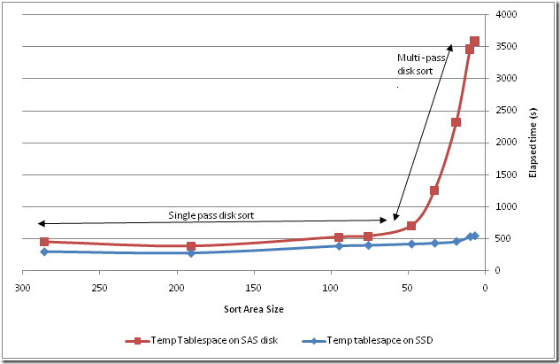
Here’s the elapsed times for various fetchsizes for the above query:

image

While the default setting of 10 is clearly better than any lower value, it’s still more than 6 times worse than a setting of 100 or 200. 

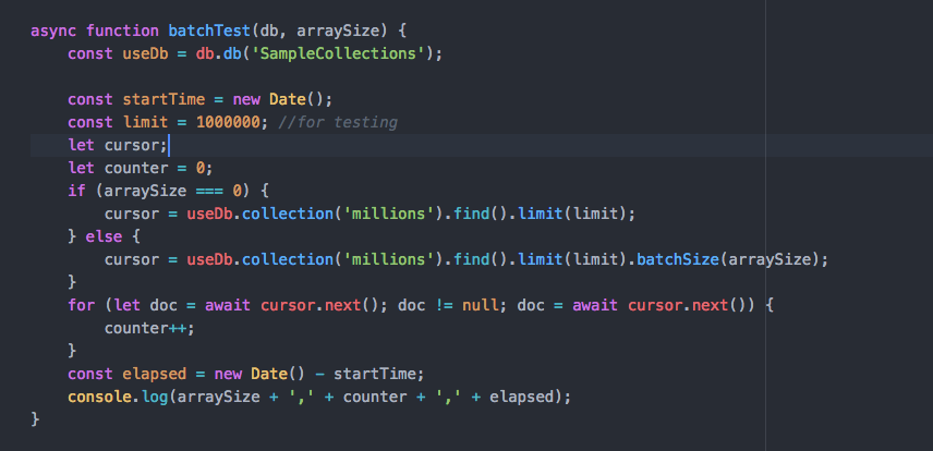
Inserting data is another situation in which we normally want to consider the array interface.  In this case we need to change our code structure a bit more noticeably.   Here’s the code we probably would write if we didn’t know about array processing:

   1:    val insSQL = "INSERT into arrayinsertTest" +
   2:        " (cust_id,cust_first_name,cust_last_name,cust_street_address) " +
   3:        " VALUES(:1,:2,:3,:4)"
   4:      val insStmt = con.prepareStatement(insSQL)
   5:      val startMs = System.currentTimeMillis
   6:      var rowCount = 0
   7:      while (rs.next()) {
   8:        insStmt.setInt(1, rs.getInt(1))
   9:        insStmt.setString(2, rs.getString(2))
  10:        insStmt.setString(3, rs.getString(3))
  11:        insStmt.setString(4, rs.getString(4))
  12:        rowCount += insStmt.executeUpdate()
  13:      }
  14:      val elapsedMs = System.currentTimeMillis - startMs
  15:      println(rowCount + " rows inserted - " + elapsedMs + " ms")
  16:      con.commit()


We prepare the statement on line 4, bind the values to be inserted on lines 8-11, then execute the insert on line 12. 

WIth a few minor changes, this code can perform array inserts:


   1:      val insSQL = "INSERT into arrayinsertTest" +
   2:        " (cust_id,cust_first_name,cust_last_name,cust_street_address) " +
   3:        " VALUES(:1,:2,:3,:4)"
   4:      val insStmt = con.prepareStatement(insSQL)
   5:      val startMs = System.currentTimeMillis
   6:      var rowCount = 0
   7:      while (rs.next()) {
   8:        insStmt.setInt(1, rs.getInt(1))
   9:        insStmt.setString(2, rs.getString(2))
  10:        insStmt.setString(3, rs.getString(3))
  11:        insStmt.setString(4, rs.getString(4))
  12:        insStmt.addBatch()
  13:        rowCount += 1
  14:        if (rowCount % batchSize == 0) {
  15:          insStmt.executeBatch()
  16:        }
  17:      }
  18:   
  19:      val elapsedMs = System.currentTimeMillis - startMs
  20:      println(rowCount + " rows inserted - " + elapsedMs + " ms")
  21:      con.commit()


On line 12, we now call the addBatch() method instead of executeUpdate().  Once we’ve added enough rows to our batch (defined by the batchsize constant in the above code) we can call executeBatch() to insert the batch. 

Array insert gives about the same performance improvements as array fetch.  For the above example I got the performance improvement below:

 Capture

To be fair, the examples above are a best case scenario for array processing – the Oracle database was running in an Amazon EC2 instance in the US, while I was running the scala code from my home in Australia!   So the round trip time was as bad as you are ever likely to see.  Nevertheless, you see pretty impressive performance enhancements from simply increasing array size in the real world all the time.

Conclusion

If you use JDBC to get data from Oracle RDBMS within a scala project, then the principles for optimization are the same as for Java JDBC – use preparedStatements, bind variables and array processing.  Of course there’s a lot more involved in optimizing database queries (SQL Tuning, indexing, etc), but these are the three techniques that vary significantly from language to language.  The performance delta from these simple techniques are very significant and should represent the default pattern for a professional database programmer. 

Using SSD for a temp tablespace on Exadata

I seem to be getting a lot of surprising performance results lately on our X-2 quarter rack Exadata system, which is good – the result you don’t expect is the one that teaches you something new.

This time, I was looking at using a temporary tablespace based on flash disks rather than spinning disks.  In the past – using Fusion IO PCI cards, I found that using flash for temp tablespace was very effective in reducing the overhead of multi-pass sorts:

image

See (http://guyharrison.squarespace.com/ssdguide/04-evaluating-the-options-for-exploiting-ssd.html)

However, when I repeated these tests for Exadata, I got very disappointing results.  SSD based temp tablespace actually lead to marginally worse performance:

image

Looking in depth at a particular point (the 500K SORT_AREA_SIZE point), we can see that although the SSD based temp tablespace has marginally better read times, it involves a significantly higher write overhead:

image

I can understand the higher read overhead (at least partially).  It’s Yet Another time when sequential write operations to an SSD device have provided disappointing performance.  However, it’s strange to see such poor read performance.  How can a spinning disk serve blocks up at effectively the same latency an SSD?

So I dumped all the direct path read waits from a 10046 trace and plotted them logarithmically:

image

We can see in this chart, that the SDD based tablespace suffers from a small “spike” of high latencies between 600-1000 us (eg .6-1 ms).  These are extremely high latencies for an SSD !  What could be causing them?  Garbage collection being caused by the almost writes to the temp tablespaces?  There was negliglbe concurrent activity on the system and the table concerned had flash cache disabled so for now that is my #1 theory. 

For that matter, why are the HDD reads times so low?  An average disk read latency of 500 us for a spinning disk is unreasonably low, is the storage cell somehow buffering temporary tablespace IO?  

As always I’m wondering if there’s someone with more expertise in Exadata internals who could shed some light on all of this!