Statistical analysis of Oracle performance data using R

R is without doubt the Open Source tool of choice for statistical analysis, it contains a huge variety of statistical analysis techniques – rivalled only by hugely expensive commercial products such as SAS and SPSS.   I’ve been playing with R a bit lately, and – of course – working with data held in Oracle.  In particular, I’ve been playing with data held in the Oracle dynamic performance views.


This post is a brief overview of installing R, connecting R to Oracle, and using R to analyse Oracle performance data.

Installing R


R can be install in linux as a standard package:

yum install R

On Windows, you may wish to use the Revolution R binaries:  http://info.revolutionanalytics.com/download-revolution-r-community.html.  I had a bit of trouble installing the 32-bit binaries on my system as they conflicted with my 64-bit JDBC.  But if you are 32-bit you might be OK.

The easiest way to setup a connection to Oracle in to install the RJDBC package.

[oracle@GuysOEL ~]$ R

R version 2.12.1 (2010-12-16)
Copyright (C) 2010 The R Foundation for Statistical Computing
ISBN 3-900051-07-0
Platform: x86_64-redhat-linux-gnu (64-bit)

<snip>

Type 'demo()' for some demos, 'help()' for on-line help, or
'help.start()' for an HTML browser interface to help.
Type 'q()' to quit R.

> install.packages("RJDBC")

Using the StatET Eclipse plug-in


I use a free eclipse plug-in called StatET.  It provides an editing environment and GUI console for the R system.  The configuration steps are a little laborious, but it has a online getting started module that guides you through the steps.  Once you have it installed, I doubt you’ll go back to the command line. 


You can get StatET at http://www.walware.de/goto/statet.  Using the eclipse environment is really handy if you’re going to use R with Oracle, since you can also use the free Toad for Eclipse extension to work on your SQLs.  Eclipse becomes a complete environment for both R and Oracle.

Getting data from Oracle into R


Once you’ve installed R, it’s pretty simple to get data out of Oracle and into R.   Here’s a very short snippet that grabs data from the V$SQL table:

   1: library(RJDBC)
   2:  
   3: drv <- JDBC("oracle.jdbc.driver.OracleDriver",
   4:                 "/ora11/home/jdbc/lib/ojdbc6.jar")
   5:  
   6: conn <- dbConnect(drv,"jdbc:oracle:thin:@hostname:1521: service","username","password")
   7: sqldata<-dbGetQuery(conn, "SELECT cpu_time cpu,elapsed_time ela,disk_reads phys,
   8:                                   buffer_gets bg,sorts sorts
   9:                              FROM V$SQL ")
  10: summary(sqldata)


Let’s look at that line by line:


Line Comments
1 The library command loads the RJDBC module, which will provide connectivity to Oracle.
3 We create a driver object for the Oracle JDBC driver.  The second argument is the location of the Oracle JDBC jar file,  almost always $ORACLE_HOME/jdbc/lib/ojdbc6.jar.
6 Connect to the Oracle database using standard JDBC connections strings
7 Create an R dataset from the result set of a query.  In this case, we are loading the contents of the V$SQL table. 
10 The R “summary” package provides simple descriptive statistics for each variable in the provided dataset.


Basic R statistical functions

R has hundreds of statistical functions,  in the above example we used “summary”, which prints descriptive statistics.  The output is shown below;  mean, medians, percentiles, etc:

image

Correlation

Statistical correlation reveals the association between two numeric variables.  If two variables always increase or decrease together the correlation is 1;  if two variables are absolutely random with respect of each other then the correlation tends towards 0.

cor prints the correlation between every variable in the data set:

image

cor.test calculates the correlation coefficient and prints out the statistical significance of the correlation, which allows you to determine if there is a significant relationship between the two variables.  So does the number of sorts affect response time?  Let’s find out:

image

The p-value is 0.19 which indicates no significant relationship – p values of no more than 0.05 (one chance in 20) are usually requires before we assume statistical significance.

On the other hand,  there is a strong relationship between CPU time and Elapsed time:

image

Plotting

plot prints a scattergram chart.  Here’s the output from plot(sqldata$ELA,sqldata$CPU):

image

Here’s a slightly more sophisticated chart using “smoothScatter”, logarithmic axes and labels for the axes:

image

Regression

Regression is used to draw “lines of best fit” between variables.  

In the simplest case, we use the “lm” package to create a linear regression model between two variables (which we call “regdata” in the example).  The summary function prints a summary of the analysis:

image

This might seem a little mysterious if your statistics is a bit rusty, but the data above tells us that there is a significant relationship between elapsed time (ELA) and physical reads (PHYS) and gives us the gradient and Y axis intercept if we wanted to draw the relationship.   We can get R to draw a graph, and plot the original data by using the plot at abline functions:

image

Testing a hypothesis


One of the benefits of statistical analysis is you can test hypotheses about your data.  For instance, what about we test the until recently widely held notion that the buffer cache hit rate is a good measure of performance.  We might suppose if that were true that SQL statements with high buffer cache hit rates would show smaller elapsed times than those with low buffer cache hit rates.  To be sure, there are certain hidden assumptions underlying that hypothesis, but for the sake of illustration let’s use R to see if our data supports the hypothesis.

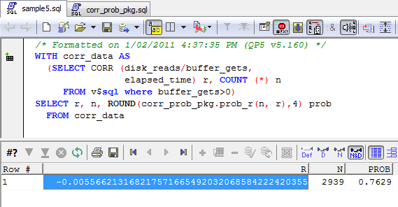
Simple correlation is a fair test for this, all we need to do is see if there is a statistically signifcant correlation between hit rate and elapsed time.  Here’s the analysis:

image

The correlation is close to 0, and the statistical significance way higher than the widely accepted .05 threshold for statistical significance.  Statements with high hit ratios do not show statistically signficantly lower elasped times that SQLs with low hit ratios.

Conclusion


There’s tons of data in our Oracle databases that could benefit from statistical analysis – not the least the performance data in the dynamic performance views, ASH and AWR.  We use statistical tests in Spotlight on Oracle to extrapolate performance into the future and to set some of the alarm thresholds.  Using R,  you have easy access to the most sophisticated statistical analysis techniques and as I hope I’ve shown, you can easily integrate R with Oracle data.

Using Toad with Hive in Amazon Elastic Map Reduce

The Toad for Cloud Databases eclipse client has support for Hive queries which makes it really easy for me to run queries against our test hadoop clusters.  It also supports Hive running on top of Amazon Elastic Map Reduce (EMR), but you do need to be aware that in EMR the default ports are different from what we have come to expect.

Firstly, if you have started an EMR cluster with Hive 0.5 support, then the Hive server will be running on port 10001, not port 10000.  The second difference is that the JobTracker is running on port 9100, rather than 50030.  So when attaching to EMR, you would set up your hive connection something like this:

1-02-2011 5-56-03 PM

Once you’ve done that, the Hive connection will show all the Hive tables and you can enter HQL queries in the SQL editor.  You can drag table and column names into the editor as well:

1-02-2011 5-57-29 PM

One of the simple, but really useful things about the hive client is that you can jump to the jobtracker web page while the HQL is running to see how it is going:

1-02-2011 5-59-19 PM

Here’s the resulting JobTracker console.  We can see the job running and – if we scroll to the right or maximize the window – we can see how the Map and reduce phases of the Hive job are progressing:

1-02-2011 8-11-07 PM

Correlation probability in Oracle

Being at the OReilly Strata conference has re-energized my inner statistic geek,  so I thought I’d share a PL/SQL package I some  years ago to calculate the probability associated with correlation coefficients calculated by Oracle.

Correlation is a statistical measure of the association between two variables.  Oracle introduced direct support for correlation in the SQL language from at least 10g (may have even been 9i).  So we can write SQL statements that calculate correlation.  So for instance,  this statement generates the correlation between the number of sorts and the elapsed times of SQL statements still cached in the SQL area:

The correlation coefficient “r” will be 1 if the two variables always increase or decrease together and –1 if one variable always increases as the other decreases.  A correlation coefficient of .33 probably represents some relationship, but anyone who has done statistics knows that you should calculate the statistical significance – chance that the result did not arise from chance – before making assertions.

Oracle doesn’t report correlation probabilities, so I implemented the formula to calculate the probability in  a PLSQL package.  It’s here.

If you pass the correlation coefficient and the number of samples (rows input to the CORR function) into the CORR_PROG_PKG.PROB_R function then it will show you the probability associated with that correlation.  So below we see the probability that this correlation is due to random fluctuation is effectively 0 (down to 4 significant figures):

Generally if the probability is less than .05 or .01 (one in 20 or 1 in 100 respectively) , then we would refer to the correlation as being statistically significant and that the two variables are related.  So we would be justified in claiming there was a relationship between sorts and elapsed time.

Just for kicks,   let’s use this technique to test the hypothesis that the Buffer Cache Hit ratio is a reliable indicator of performance.  Here’s the result:

The correlation is very low and the probability that there is no association is very high – way above the .05 probability.  In other words, in this database there is no statistically significant relationship between the elapsed time of an SQL and it’s buffer cache hit rate!

Working with Cassandra 0.7

In this post,  I experimented with inserting data from Oracle into Cassandra column families using Hector.  Unfortunately, that code isn’t compatible with the latest Cassandra 0.7 release, so I had to rework it.  The new version uses the addInsertion method of the Mutator object and while not totally intuitive didn’t take long to get working.  Here are the key changes:

   1: private static void insertSales(Connection oracleConn, Keyspace keyspace,
   2:         String cfName) throws SQLException {
   3:     int rows = 0;
   4:     ColumnPath cf = new ColumnPath(cfName);
   5:     Statement query = oracleConn.createStatement();
   6:  
   7:     String sqlText = "SELECT cust_id, cust_first_name,  cust_last_name, prod_name, "
   8:             + "           SUM (amount_sold) sum_amount_sold,sum(quantity_sold) sum_quantity_sold "
   9:             + "          FROM sh.sales    "
  10:             + "          JOIN sh.customers USING (cust_id) "
  11:             + "          JOIN sh.products  USING (prod_id)  "
  12:             + "         GROUP BY cust_id, cust_first_name,  cust_last_name,  prod_name "
  13:             + "         ORDER BY cust_id, prod_name ";
  14:     ResultSet results = query.executeQuery(sqlText);
  15:     int rowCount = 0;
  16:     int lastCustId = -1;
  17:     while (results.next()) { // For each customer
  18:         Integer custId = results.getInt("CUST_ID");
  19:         String keyValue = custId.toString();
  20:  
  21:         if (rowCount++ == 0 || custId != lastCustId) { // New Customer
  22:             String custFirstName = results.getString("CUST_FIRST_NAME");
  23:             String custLastName = results.getString("CUST_LAST_NAME");
  24:             System.out.printf("%s %s\n", custFirstName, custLastName);
  25:             // Create a supercolumn for customer details (first, lastname)
  26:             Mutator<String> mutator = HFactory.createMutator(keyspace,
  27:                     stringSerializer);
  28:             mutator.addInsertion(keyValue, cfName, HFactory
  29:                     .createSuperColumn("CustomerDetails", Arrays
  30:                             .asList(HFactory.createStringColumn(
  31:                                     "customerFirstName", custFirstName)),
  32:                             StringSerializer.get(), StringSerializer.get(),
  33:                             StringSerializer.get()));
  34:             mutator.addInsertion(keyValue, cfName, HFactory
  35:                     .createSuperColumn("CustomerDetails", Arrays
  36:                             .asList(HFactory.createStringColumn(
  37:                                     "customerLastName", custLastName)),
  38:                             StringSerializer.get(), StringSerializer.get(),
  39:                             StringSerializer.get()));
  40:  
  41:             mutator.execute();
  42:         }
  43:         // Insert product sales total for that customer
  44:         String prodName = results.getString("PROD_NAME");
  45:         Float SumAmountSold = results.getFloat("SUM_AMOUNT_SOLD");
  46:         Float SumQuantitySold = results.getFloat("SUM_QUANTITY_SOLD");
  47:         // Supercolumn name is the product name
  48:         Mutator<String> mutator = HFactory.createMutator(keyspace,
  49:                 stringSerializer);
  50:         mutator.addInsertion(keyValue, cfName, HFactory.createSuperColumn(
  51:                 prodName, Arrays.asList(HFactory.createStringColumn(
  52:                         "AmountSold", SumAmountSold.toString())),
  53:                 StringSerializer.get(), StringSerializer.get(),
  54:                 StringSerializer.get()));
  55:         mutator.addInsertion(keyValue, cfName, HFactory.createSuperColumn(
  56:                 prodName, Arrays.asList(HFactory.createStringColumn(
  57:                         "QuantitySold", SumQuantitySold.toString())),
  58:                 StringSerializer.get(), StringSerializer.get(),
  59:                 StringSerializer.get()));
  60:         mutator.execute(); 
  61:         lastCustId = custId;
  62:         rows++;
  63:     }
  64:     System.out.println(rows + " rows loaded into " + cf.getColumn_family());
  65: }

The reason why I wanted to do this was to play with Cassandra using our (relatively) new Toad for Cloud Databases Eclipse client.  Toad for Cloud Databases lets you work with non-relational datasources such as Cassandra, HBase, SimpleDB, etc, using SQL.   

Here’s how it works.  We select the column family we want to map from the Cassandra server:

14-01-2011 3-21-00 PM Map Cassandra1

That column family contains data loaded from both the Oracle CUSTOMER and SALES tables.   Toad recognizes that the data in that single column family is best represented by two normalized tables,  and gives us the opportunity to specify the names for the primary and foreign keys.  We can also rename the “tables” (more like views really) that Toad will create:

14-01-2011 3-22-34 PM map cassandra2

The resulting tables look similar to the tables that we originally loaded from Oracle, and we can issue SQL queries against them just as we could have with Oracle.  The queries get translated from SQL to thrift calls against the underlying Cassandra Server:

14-01-2011 4-16-50 PM cassandra query

I definitely find it easier to issue SQL than write a 200 line Java program to do the same thing!  Of course, I'm not much of a Java programmer, but at a minimum having Toad to query the Cassandra data is invaluable when checking to see that your program did was it was intended to do 

Accelerating Oracle database performance with SSD

I was recently asked to provide advice on how best to accelerate Oracle database performance with flash SSD.   In this post I’ll attempt to outline some thoughts on that.

There’s some thinking that SSD will soon replace spinning disk altogether - we just have to wait for the price to come down.  However, I’m not so sure that this complete replacement is likely to occur in the immediate future.   There are two competing forces at work:

  • The economies of “big data”, which drive us to reduce the cost per unit of storage ($$/TB):   magnetic disk costs only about 5% of the cost of a high end SSD per terabyte.
  • The economies of high IO throughput, in which we are motivated to reduce the cost of providing a given IO rate.  SSD (PCi flash) can generate IO rates at 1/20th of the cost of magnetic disks.

These two competing economies are not likely to change in the immediate future:  magnetic disk can store large amounts of data much more cheaply than SSD;  SSD can deliver very high IO rates more cheaply than magnetic disk.  For most databases, it will not be cost effective to place the entire database on SSD – the best outcome will be obtained when we place parts of the database on SSD and some on magnetic disk.

SSD Performance basics

I’ve posted in the past on how SSD works with the Oracle flash cache,  and I’ve presented on SSD performance at OOW.  You might like to review those items.  However,  here’s a quick review of the basics:

  • All flash drives offer pretty good read performance – say 25 microseconds for a single page read
  • When inserting data into an empty page, performance is slower, but not awful – around 250 microseconds
  • In order to update an existing page, a block erase is required – much, much slower – maybe 2000 microseconds

image

Enterprise SSD vendors - Fusion IO, Virident, etc - all have sophisticated algorithms to avoid the write penalty associated with SSD block erase operations.  Amongst other techniques, they will maintain a pool of unused blocks.  When a page needs to be updated it will be marked as invalid in the original location and moved to one of these blocks.  Later on, garbage collection routines will clear up the invalid entries.  The result is that updates don't always have to incur the high overhead of block erase operations.

Nevertheless, you want to avoid placing write intensive files on a flash disk, because as the disk fills up with modified blocks - and especially if the write rate exceeds the garbage collection capabilities - you might see the disk slow down dramatically.

To summarize:

Flash-based disks perform reads much faster than writes, and can suffer from performance degradation if subjected to intensive sustained write operations.


Options for SSD deployment on Oracle


Given the performance characteristics of SSD,  how best to use SSD to boost Oracle performance?  There are a few options:

  • Put the entire database on SSD
  • Place selected segments on SSD
  • Use the 11GR2 flash cache
  • Put temporary tablespace on SSD
  • Put the redo logs on SSD

Let’s look at each of these in turn:

Put the entire Database on SSD

This works great – if you can afford it.  For most databases the cost of putting it all on SSD is too high.  Placing data that is rarely accessed on SSD is not very cost effective, because you are paying a high cost per GB, but not getting any benefit from the relatively cheap IO rates. 

Place selected segments on SSD

This is probably the best option if you don’t have enough SSD for the entire database, but it does require a bit of configuration.   We identify the segments with the most IO,  perhaps using a query on V$SEGMENT_STATISTICS:


We are looking for object that have a high read/write ratio, contribute to a significant number of reads, and are small enough to fit on our SSD.   We create a tablespace on SSD, then move these objects to that tablespace.

If our most read intensive tables are massive, then they might not fit on the SSD.  In this case we could consider partitioning them and placing the hottest partitions on SSD.  

Use the 11GR2 flash cache

If you have 11GR2 and are on a compatible platform (Solaris or Oracle Enterprise Linux), then you can setup the Oracle DB flash cache.  This is absolutely the easiest option – all you need to do is set a few parameters and bounce the database.  The flash cache automatically caches the hottest blocks and usually provides an excellent performance improvement.

The improvement is not as significant as moving objects directly onto flash storage, since there still has to be magnetic disk IO getting things on and off.  Also, the architecture tends to create a lot of writes to the SSD, which can challenge garbage collection.  The chart below sums up a typical outcome – a huge boost from the flash cache, but not as big a boost as we could get by putting objects directly on SSD:

image

Put temporary tablespace on SSD


Temporary tablespace IO (from sorts and hash operations) can sometimes be the most significant form of database IO, and often the entire temporary tablespace will fit on the SSD.  So should we consider putting temporary tablespace on the SSD?

I’m a bit reluctant to do this:  by definition temporary tablespace IO is equal parts reads and writes, and since we are motivated to avoid write IO to the SSD, this seems like a dubious option.  However, if your performance is absolutely dominated by temp tablespace IO and your SSD is tolerant of high write rates (eg has excellent garbage collection,etc) then it might be worth trying.  After all,  the SSD will definitely speed up the read side of temporary tablespace IO, even if the write IO does not get a significant boost. 

Put redo logs on SSD

Although redo logs are very IO intensive, it’s almost all write IO and therefore this is probably not the best option.   During sustained writes the Garbage Collection will probably break down and the disk might not end up performing that much better than a spinning disk.  I'd not recommend this. 

Conclusions


You can use SSD to boost database performance even if you don’t have enough for the entire database.  Best options are:

  1. Place segments with high read but low write rates directly on SSD
  2. Use the SSD with the 11GR2 database flash cache (if you are on OEL or Solaris)
  3. If temporary segment IO is absolutely your bottleneck – but only then – consider placing the temporary tablespace on SSD.

I don’t think using SSD for redo logs is a good idea.  The high rates of sustained sequential write IO is not the ideal type of IO for SSD.

Gearing up for OOW 2010

It’s that time of the year again,  and as always I’m looking forward (really!) to Oracle Open World.  I’ve been every year since 1998 and this year looks like being the biggest ever – which boggles the imagination considering how big last year was!

This year I’m giving two technical sessions, hosting an unconference, doing a book signing and – together with the inimitable Steven Feuerstein, hosting a Quest evening event.   In between that I hope to attend as many sessions as I can and catch up with friends a colleagues.  Here are the details of my sessions and other appearances:

Tuesday  11:00 am - Hadoop & NoSQL unconference session

Mason room, PARC55, 55 Cyril Magnin Street 

Unconference sessions are run by the attendees and are Powerpoint-free.  I proposed this one to get together with others who are interested in Hadoop and NoSQL databases. 

Tuesday 3:00 pm - “Oracle Performance Survival Guide” book signing 

Quest booth # 1421 – Moscone South Hall 
I’ll be signing and giving away copies of my book Oracle Performance Survival Guide at the Quest booth.  

Tuesday  5:30pm – 7pmQuest evening with the experts 

AMC Metreon Movie Theater ,101 4th Street

Steven Feuerstein and I will be hosting an evening with the experts with a special presentation and live Q&A.  Refreshments will be provided.

Thursday 09:00 am S313603:  Solid-State Disk and the Oracle Database 11g Release 2 Flash Cache

Moscone South, Room 307

Solid State disk changes the physics of database performance in really exciting ways.  DBAs should get familiar with SSD technologies so they can make sensible decisions about using SSD with Oracle.  I’ll be talking about the mechanics of SSD, including things like garbage collection, wear-leveling, PCI vs SATA and so on.  Then we’ll look at how the 11GR2 flash cache works and when you might want to use it.

Thursday  12:00 Noon S314916 : Optimizing Oracle Databases on VMware

Moscone South, Room 302

This presentation summarizes what we’ve learned at Quest about optimizing Oracle databases running in VMWare environments, particularly ESX.  I’ll be talking about CPU, memory and disk configuration for ESX and also the differences between ESX and Oracle VM and why that difference matters. 

Oracle tables vs Cassandra SuperColumns


In my last post,  I wrote some Java code to insert Oracle tables into Cassandra column families.  As much fun as this was for me, it was  fairly trivial and not a particularly useful exercise in terms of learning Cassandra. 

In Cassandra,  data modelling is very different from the relational models we are used to and one would rarely convert a complete Oracle schema from tables directly to ColumnFamilies .  Instead, Cassandra data modelling involves the creation of ColumnFamilies with SuperColumns to represent master-detail structures that are commonly referenced together

SuperColumns vs Relational schema


At the Cassandra Summit in August,  Eben Hewitt gave a presentation on Cassandra Data Modelling.   There’s a lot of nuance in that talk and in the topic, but a key point in Cassandra – as in many other NoSQL databases – is that you model data to match the queries you need to satisfy,  rather than to a more theoretically "pure" normalized form.   For relational guys, the process is most similar to radical denormalization in which you introduce redundancy to allow for efficient query processing.

For example, let’s consider the Oracle SH sample schema.  Amongst other things, it includes SALES, PRODUCTS and CUSTOMERS:


9-09-2010 3-35-32 PM Oracle sample schema

We could map each Oracle table to a Cassandra ColumnFamily, but because there are no foreign key indexes or joins,  such a Cassandra data model would not necessarily support the types of queries we want.  For instance, if we want to query sales totals by customer ID, we should create a column family keyed by customer id, which contains SuperColumns named for each product which in turn includes columns for sales totals.  It might look something like this:

ID CustomerDetails Product Name #1 Product Name #2 ………….. Product Name #N
1
First Name Last Name
Guy Harrison
Quantity Value
3 $100,020
  …………..
Quantity Value
3 $130,000
2
First Name Last Name
Greg Cottman
 
Quantity Value
34 $10,080
…………..
Quantity Value
4 $99,000


Each customer “row” has super column for each product that contains the sales for that product.  Not all customers have all the supercolumns - each customer has supercolumns only for each product they have purchased.  The name of the SuperColumn is the name of the product.  

Giving the column the name of the product is a major departure from how we would do things in Oracle.  The name of a column or SuperColumn can be determined by the data, not by the schema - a concept completely alien to relational modelling.

Inserting into SuperColumns with Hector


To try and understand this,  I created a Cassandra columnfamily of the type “Super”.  Here’s my definition in the storage-conf.xml file:

<ColumnFamily Name="SalesByCustomer" 
ColumnType="Super"
CompareWith="UTF8Type"
CompareSubcolumnsWith="UTF8Type"
Comment="Sales summary for each customer "/>

And here is some of my Hector Java program, which reads sales totals for each customer from the Oracle sample schema, and inserts them into the ColumnFamily:

   1: private static void insertSales(Connection oracleConn, Keyspace keyspace,
   2:         String cfName) throws SQLException {
   3:     int rows = 0;
   4:     ColumnPath cf = new ColumnPath(cfName);
   5:     Statement query = oracleConn.createStatement();
   6:  
   7:     String sqlText = "SELECT cust_id, cust_first_name,  cust_last_name, prod_name, "
   8:             + "           SUM (amount_sold) sum_amount_sold,sum(quantity_sold) sum_quantity_sold "
   9:             + "          FROM sh.sales    "
  10:             + "          JOIN sh.customers USING (cust_id) "
  11:             + "          JOIN sh.products  USING (prod_id)  "
  12:             + "         GROUP BY cust_id, cust_first_name,  cust_last_name,  prod_name "
  13:             + "         ORDER BY cust_id, prod_name ";
  14:     ResultSet results = query.executeQuery(sqlText);
  15:     int rowCount = 0;
  16:     int lastCustId = -1;
  17:     while (results.next()) { // For each customer
  18:         Integer custId = results.getInt("CUST_ID");
  19:         String keyValue = custId.toString();
  20:  
  21:         if (rowCount++ == 0 || custId != lastCustId) { // New Customer
  22:             String custFirstName = results.getString("CUST_FIRST_NAME");
  23:             String custLastName = results.getString("CUST_LAST_NAME");
  24:             System.out.printf("%s %s\n", custFirstName, custLastName);
  25:             //Create a supercolumn for customer details (first, lastname)     
  26:             cf.setSuper_column(StringUtils.bytes("CustomerDetails"));
  27:             cf.setColumn(StringUtils.bytes("customerFirstName"));
  28:             keyspace.insert(keyValue, cf, StringUtils.bytes(custFirstName));
  29:             cf.setColumn(StringUtils.bytes("customerLastName"));
  30:             keyspace.insert(keyValue, cf, StringUtils.bytes(custLastName));
  31:         }
  32:         //Insert product sales total for that customer 
  33:         String prodName = results.getString("PROD_NAME");
  34:         Float SumAmountSold = results.getFloat("SUM_AMOUNT_SOLD");
  35:         Float SumQuantitySold = results.getFloat("SUM_QUANTITY_SOLD");
  36:         //Supercolumn name is the product name 
  37:         cf.setSuper_column(StringUtils.bytes(prodName));
  38:         cf.setColumn(StringUtils.bytes("AmountSold"));
  39:         keyspace.insert(keyValue, cf, StringUtils.bytes(SumAmountSold.toString()));
  40:         cf.setColumn(StringUtils.bytes("QuantitySold"));
  41:         keyspace.insert(keyValue, cf, StringUtils.bytes(SumQuantitySold.toString()));
  42:         
  43:         lastCustId = custId;
  44:         rows++;
  45:     }
  46:     System.out.println(rows + " rows loaded into " + cf.getColumn_family());
  47: }

This code is fairly straightforward,  but let’s step through it anyway:

Lines Description
7-14 Execute the Oracle SQL to get product summaries for each customer
17 Loop through each row returned (one row per product per customer)
21 Check to see if this is a completely new customer
26-30 If it is a new customer,  create the CustomerDetails SuperColumn for that customer.  The SuperColumn name is “CustomerDetails” and it contains columns for Firstname and Lastname.
37-41

Now we create a SuperColumn for a specfic product, still keyed to the customer.  The SuperColumn name is set to the name of the product (line 37).  Inside the supercolumn are placed columns “AmountSold” (lines 38-39) and “QuantitySold” (lines 40-41)


Querying SuperColumns


Inserting master detail relationships into a supercolumn column family was easy enough.  I had a lot more difficulty writing code to query the data.  The tricky part seems to be when you don’t know the name of the SuperColumn you want to read from.  There's no direct equivalent to the JDBC ResultMetaData object to query the SuperColumn names - instead you create a "SuperSlice" predictate that defines a range of SuperColumns that you want to retrieve.  It's a bit awkward to express the simple case in which you want to return all the SuperColumns. 

Below is a bit of code which retrieves sales totals for a specific customer id.  I suspect I've made a few newbie mistakes :-):

   1: public static void querySuperColumn(Keyspace keyspace, String cfName,
   2:         String keyValue) {
   3:  
   4:     ColumnPath colFamily = new ColumnPath(cfName);
   5:     System.out.println("Details for customer id " + keyValue);
   6:  
   7:     /* Get Customer Details */
   8:     colFamily.setSuper_column(StringUtils.bytes("CustomerDetails"));
   9:     SuperColumn custDetailsSc = keyspace
  10:             .getSuperColumn(keyValue, colFamily);
  11:     for (Column col : custDetailsSc.getColumns()) {
  12:         String colName = StringUtils.string(col.getName()); 
  13:         String colValue = StringUtils.string(col.getValue()); 
  14:         System.out.printf("\t%-20s:%-20s\n", colName, colValue);
  15:     }
  16:     /* Get dynamic columns -  */
  17:     ColumnParent colParent = new ColumnParent(cfName);
  18:     SliceRange sliceRange = new SliceRange(StringUtils.bytes(""), StringUtils
  19:             .bytes(""), false, 2 ^ 32); // TODO: what if there are > 2^32 ??                                             
  20:     SlicePredicate slicePredicate = new SlicePredicate();
  21:     slicePredicate.setSlice_range(sliceRange);
  22:     //TODO:  Surely there's an easier way to select all SC than the above??
  23:     List superSlice = keyspace.getSuperSlice(keyValue,
  24:             colParent, slicePredicate);
  25:     for (SuperColumn prodSuperCol : superSlice) {  //For each super column
  26:         String superColName = StringUtils.string(prodSuperCol.getName());
  27:         if (!superColName.equals("CustomerDetails")) { // Already displayed
  28:                                                          
  29:             System.out.printf("\n%50s:", superColName); // product Name 
  30:             List columns1 = prodSuperCol.getColumns();
  31:             for (Column col : columns1) {               // product data 
  32:                 String colName = StringUtils.string(col.getName()); 
  33:                 String colValue = StringUtils.string(col.getValue()); 
  34:                 System.out.printf("\t%20s:%-20s", colName, colValue);
  35:  
  36:             }
  37:         }
  38:     }
  39:  
  40: }
Lines Description
8-9 Set the superColumn to the “CustomerDetails” supercolumn
11-14 Retrieve the column values (firstname, surname) for the CustomerDetails supercolumn
17-21 Set up a “SlicePredicate” that defines the supercolumns to be queried.  I want to get all of the supercolumns (eg every product), so I set up an unbounded range (line 18) and supply that to the slice predicate (line 21)
23 Create a list of supercolumns.  This will include all the SuperColumns in the column family (including, unfortunately,  CustomerDetails)
27 Eliminate CustomerDetails from the result.  Here we only want product names
30-35 Iterate through the columns in each supercolumn.  THis will extract QuantitySold and AmountSold for each Product name


Here’s some output from the Java program.  It prints out customer Details and product sales totals for customer# 10100:

Details for customer id 101000
customerFirstName :Aidan
customerLastName :Wilbur

CD-RW, High Speed Pack of 5: AmountSold:11.99 QuantitySold:1.0
Keyboard Wrist Rest: AmountSold:11.99 QuantitySold:1.0
Multimedia speakers- 3" cones: AmountSold:44.99 QuantitySold:1.0


SuperColumns with Toad for Cloud Databases 


Toad for cloud databases now has Cassandra support, which makes querying SuperColumns s a lot easier.  SuperColumns that have dynamic names but uniform internal column structure (as in my example above) are represented by Toad for Cloud Databases as a detail table.  To put it another way,  Toad for Cloud Databases re-normalizes the data - displaying it in the format that we would typically use in an RDBMS. 

So when we point Toad for Cloud databases at our SalesByCustomer column family, it maps the column family to two tables:  one for CustomerDetails and the other - which by default it will call SalesByCustomersuper_column” – for product sales totals.  We can rename the subtable and subtable key during the mapping phase to make it clearer that it represents product details.

9-09-2010 1-56-19 PM map cassandra super col

Now if we want to extract product details for a particular customer, we can do a SQL join.  Below we build the join in the query builder, but of course we could simply code the SQL by hand as we would for any NoSQL or SQL database supported by Toad for Cloud Databases:

9-09-2010 3-49-36 PM cassandra supercol qry

And just to close the loop, here we can see that the Toad for Cloud databases query returns the same data as the Hector query:

9-09-2010 3-50-48 PM cassabdra supercol results


Conclusion


All NoSQL databases require that we change the way we think about data modelling, and Cassandra is no exception.  SuperColumns are an incredibly powerful construct, but I can’t say that I found them intuitive or easy.  Hopefully APIs and tooling will evolve to make life easier for those of us coming from the relational world.

Playing with Cassandra and Oracle

Cassandra  is one of the hottest of the NoSQL databases.  From a production DBAs perspective it’s not hard to see why:  while some of the other NoSQLs offer more programming bells and whistles for the developer, Cassandra is built from the ground up for total and transparency redundancy and scalability, close to the heart of every DBA.

However,  Cassandra involves some complex data modelling concepts – mainly around the notorious SuperColumn concept, and I don’t think I’ll ever understand it fully until I’ve played directly with some data.  To that end, I thought I’d start by trying to model some familiar Oracle sample schemas in Cassandra.

Toad for Cloud Databases is releasing support for Cassandra early next month (eg September 2010), so I’ve been using that – as well as Java of course – to try to get some initial data loaded.

For other NoSQL databases,  Toad for Cloud lets us create NoSQL tables from relational tables with a couple of clicks.  Unfortunately, we can’t do that with Cassandra, since you can’t create a ColumnFamily on the fly.  So my first Cassandra tasks was to write a simple program to take an Oracle table (or query) and create a matching column family.

Getting started

Getting started with Cassandra was surprisingly easy.  I followed the instructions in http://schabby.de/cassandra-installation-configuration/ to install Cassandra on my laptop, and installed the hector Java interface from http://prettyprint.me/2010/02/23/hector-a-java-cassandra-client/.

Terminology in NoSQL can be confusing, with each NoSQL database using terms differently from each other, and all of them using terms differently from RDBMS.  In Cassandra:

  • A Keyspace is like a schema
  • ColumnFamily is roughly like a table

Things get very funky when SuperColumns are introduced, but lets skip that for now.

To create a ColumnFamily in Cassandra 0.6, we have to add its name to the storage-conf.xml file which is in the Conf directory and then restart Cassandra.  In 0.7 there’ll be a way to do this without restarting the server.

Here is where I created a keyspace called “Guy” and created some ColumnFamilies to play with:

   1: "Guy">
   2:   "G_Employees" CompareWith="UTF8Type"/>
   3:   "G_Employees2" CompareWith="UTF8Type"/>
   4:   "G_Employees3" CompareWith="UTF8Type"/>
   5:   org.apache.cassandra.locator.RackUnawareStrategy
   6:   1
   7:   org.apache.cassandra.locator.EndPointSnitch
   8: 


Loading data


I wrote some Java code that takes a SQL statement, and loads the result set directly into a column family.  Here’s the critical method (the complete java program with command line interface is here):

   1: private static void oracle2Cassandra(Connection oracleConn,
   2:         Keyspace keyspace, String cfName, String sqlText)
   3:         throws SQLException {
   4:     int rows = 0;
   5:     ColumnPath cf = new ColumnPath(cfName);
   6:     Statement oraQuery = oracleConn.createStatement();
   7:     ResultSet result = oraQuery.executeQuery(sqlText);
   8:     ResultSetMetaData rsmd = result.getMetaData();
   9:     while (result.next()) { // For each row in the output
  10:         // The first column in the result set must be the key value
  11:         String keyValue = result.getString(1);
  12:         // Iterate through the other columns in the result set
  13:         for (int colId = 2; colId <= rsmd.getColumnCount(); colId++) {
  14:             String columnName = rsmd.getColumnName(colId);
  15:             String columnValue = result.getString(colId);
  16:             if (!result.wasNull()) {
  17:             cf.setColumn(StringUtils.bytes(columnName));
  18:                 keyspace.insert(keyValue, cf, StringUtils
  19:                         .bytes(columnValue));
  20:             }
  21:         }
  22:         rows++;
  23:     }
  24:     System.out.println(rows + " rows loaded into " + cf.getColumn_family());
  25: }

The method take s a Oracle connection and a SQL statement, and pushes the data from that SQL into the Cassandra column family and keyspace specified.   The first column returned by the query is used on the key to the Cassandra data.

Lines 6-8 execute the statement and retrieve a ResultSet object – which contains the data – and a ResultSetMetaData object which contains the column names.  Lines 9-21 just iterate through the rows and columns and create entries in the Column Family that match.   We use the Hector setColumn methodto set the name of the column and the insert method to apply the column value.  Too easy!

Of course, I’d have no idea as to whether my job had worked if I didn’t have Toad for Cloud databases available.  Using TCD, I can map the Cassandra columnFamily to a TCD “table” and browse the table (eg Cassandra Column Family) to see the resulting data:

image

I can even use SQL to join the Cassandra data to the Oracle data to make absolutely certain that the data transfer went OK:

image


It’s surprisingly easy to get started with Cassandra.  Installation of a test cluster is a breeze, and the Hector Java API is straight forward.    Of course,  direct mapping of RDBMS tables to Cassandra ColumnFamilies doesn’t involve the complexities of advanced Cassandra data models using variable columns and SuperColumns.    Next, I’m going to try and map a more complex ColumnFamily which maps to multiple Oracle tables – hopefully won’t make my brain hurt too much!

Toad for Cloud Databases is introducing Cassandra support in the 1.1 release due out within the next two weeks.  Its a free download from toadforcloud.com

“Stolen” CPU on Xen-based virtual machines

I’ve written previously about how VMWare ESX manages CPU and how to measure your“real” CPU consumption if you are running an database in such a VM. 

VMware is currently the most popular virtualization platform for Oracle database virtualization, but Oracle’s own Oracle Virtual Machine uses the open source Xen hypervisor, as does Amazon’s Elastic Compute Cloud (EC2): which runs quite a few Oracle databases.    So Oracle databases – and many other interesting workloads – will often be found virtualized inside a Xen-based VM.

I recently discovered that there is an easy way to view CPU overhead inside a Xen VM, at least if you are running a paravirtulized linux kernel 2.6.11 or higher.

Read More

Consistency models in Non relational Databases

One of the most significant differences between the new generation of non-relational (AKA NoSQL) databases and the traditional RDBMS is the way in which consistency of data is handled.  In a traditional RDBMS, all users see a consistent view of the data.  Once a user commits a transaction, all subsequent queries will report that transaction and certainly no-one will see partial results of a transaction.

RDBMS transactions are typically described as “ACID” transactions.  That is, they are:

  • Atomic: The transaction is indivisible – either all the statements in the transaction are applied to the database, or none are.
  • Consistent: The database remains in a consistent state before and after transaction execution.
  • Isolated: While multiple transactions can be executed by one or more users simultaneously, one transaction should not see the effects of other concurrent transactions.
  • Durable: Once a transaction is saved to the database (an action referred to in database programming circles as a commit), its changes are expected to persist.

As databases become distributed across multiple hosts,  maintaining ACID consistency becomes increasingly difficult.  In a transaction that spans multiple independent databases, complex two-phase commit protocols must be employed.  In the case of a truly clustered distributed database even more complex protocols are required, since the state of data in memory and the state of data in various transaction logs and data files must be maintained in a consistent state (cache fusion in Oracle RAC for instance).

CAP Theorem:  You can’t have it all


In 2000,  Eric Brewer outlined the CAP (AKA Brewer’s) Theorem.   Simplistically,  CAP theorem says that in a distributed database system, you can only have at most two of the following three characteristics:

  • Consistency: All nodes in the cluster see exactly the same data at any point in time
  • Availability: Failure of a node does not render the database inoperative
  • Partition tolerance:  Nodes can still function when communication with other groups of nodes is lost

Text Box-Quest Blue

Interpretation and implementations of CAP theorem vary,  but most of the NoSQL database system architectures favour partition tolerance and availability over strong consistency.

Eventual Consistency


A compromise between eventual consistency and weak (no guarantees) consistency is Eventual Consistency.

The core of the eventual consistency concept is that although the database may have some inconsistencies at a point in time, it will eventually become consistent should all updates cease.  That is,  inconsistencies are transitory:  eventually all nodes will receive the latest consistent updates.

BASE – Basically Available Soft-state Eventually consistent is an acronym used to contrast this approach with the RDBMS ACID transactions described above.

Not all implementations of eventually consistent are equal.     In particular, an eventually consistent database may also elect to provide the following:

  • Causal consistency:  This involves a signal being sent from between application sessions indicating that a change has occurred.  From that point on the receiving session will always see the updated value.
  • Read your own writes:  In this mode of consistency, a session that performs a change to the database will immediately see that change, even if other sessions experience a delay.
  • Monotonic consistency:  In this mode, A session will never see data revert to an earlier point in time.   Once we read a value, we will never see an earlier value.   


The NRW notation

NRW notation describes at a high level how a distributed database will trade off consistency, read performance and write performance.  NRW stands for:

  • N: the number of copies of each data item that the database will maintain. 
  • R: the number of copies that the application will access when reading the data item 
  • W: the number of copies of the data item that must be written before the write can complete.  

When N=W then the database will always write every copy before returning control to the client – this is more or less what traditional databases do when implementing synchronous replication.   If you are more concerned about write performance than read performance, then you can set W=1, R=N.  Then each read must access all copies to determine which is correct, but each write only has to touch a single copy of the data.

Most NoSQL databases use N>W>1:  more than one write must complete, but not all nodes need to be updated immediately.   You can increase the level of consistency in roughly three stages:

  1. If R=1, then the database will accept whatever value it reads first.  This might be out of date if not all updates have propagated through the system.   
  2. If R>1 then the database will more than one value and pick either the most recent (or “correct”) value.
  3. If W+R>N, then a read will always retrieve the latest value,  although it may be mixed in with “older” values.  In other words, the number of copies you write and the number of copies you read is high enough to guarantee that you’ll always have at least one copy of the latest version in your read set.   This is sometimes referred to as quorum assembly. 
     
NRW configuration Outcome
W=N  R=1 Read optimized strong consistency
W=1 R=N Write optimized strong consistency
W+R<=N Weak eventual consistency.  A read might not see latest update
W+R>N Strong consistency through quorum assembly.  A read will see at least one copy of the most recent update


NoSQL databases generally try hard to be as consistent as possible, even when configured for weaker consistency.  For instance, the read repair algorithm is often implemented to improve consistency when R=1.  Although the application does not wait for all the copies of a data item to be read,  the database will read all known copies in the background after responding to the initial request.  If the application asks for the data item again, it will therefore see the latest version. 

Vector clocks

NoSQL databases can seem simplistic in some respects, but there’s a lot of really clever algorithms going on behind the scenes.   For example,  the vector clock algorithm can be used to ensure that updates are processed in order (monotonic consistency).

With vector clocks,  each node participating in the cluster maintains an change number (or event count) similar to the System Change Number used in some RDBMSs.  The “vector” is a list including the current node's change number as well as the change numbers that have been received from other nodes.  When an update is transmitted, the vector is included with the update and the receiving node compares that vector with other vectors that have been received to determine if updates are being received out of sequence.    Out of sequence updates can be held until the preceding updates appear.

I found vector clocks hard to understand until I read the description in Operating Systems: Concurrent and Distributed Software Design  by Jean Bacon and Tim Harris (Addison-Wesley).

Amazon’s Dynamo

A lot of the eeventually consistent concepts were best articulated by Amazon in Verner Vogels’ Eventually Consistent paper and in Amazon’s paper on the Dynamo eeventually consistent key-value store.   Dynamo implements most of the ideas above, and is the inspiration for several well known NoSQL datastores including Voldemort and – together with Google’s BigTable specification – Cassandra.


Cloud (AKA NoSQL) Databases and me

I’ve been an RDBMS guy now since about 1988.    Around the time my first son Chris was born, the government department were I worked shifted from an ADABAS/MVS environment to an Oracle/VMS system, and I was dropped headfirst into joy of Oracle 5.1.  Since then I’ve been continuously involved with Oracle development, administration and performance as well in Sybase, MySQL and SQL Server.  So you could say I’m a pretty hard core old-school SQL database guy.

For the longest time, it looked like the RDBMS was here to stay.  But a few years ago,  we noticed signs of new models for databases that were better aligned with modern application architectures,  the massive “big data” demands of Web 2.0 and the increasing disparity between IO and CPU capabilities.   I’ve written and talked  about some of these trends over the past two years and I’ve placed some links to those articles the end of this post. 

What I haven’t been able to talk much about is what we are doing to support these Cloud/NoSQL database at Quest Software.   Quest is  diverse company, with strong offerings in Applications, Virtualization and Windows management,  but we are definitely very dominant in database tools, so you might have been wondering how we planned to move into the next generation of database management tools.  

For the past year or so,  I’ve been directing a team of developers who are building “Toad for Cloud Databases” which will provide data management capabilities for NoSQL/Cloud databases in a familiar TOAD platform.   This Toad will allow developers, DBA and Data analysts to work with data in these databases just as easily as you would with data in an RDBMS.  Even better, you’ll be able to move data between RDBMS and a NoSQL/Cloud database, and issue queries that join data in both databases. 

I can’t say much more about Toad for Cloud Databases in advance of it’s official release later this month.  But I will be starting to blog more frequently on NoSQL topics,  both in this blog and in the Toad for Cloud Databases community site that will be active my the end of June.

In this personal blog,  I’m going to publish some summaries of the things we’ve learned about the various NoSQL/Cloud Databases, especially from the perspective of an RDBMS professional.  I’ll also be posting early versions of articles and posting that will eventually go up on the official Toad for Cloud website.

I’m pretty excited about what we’re doing with Toad for Cloud Databases, and I’m looking forward to sharing some of this stuff with you.  Of course,  we’re still busily working on RDBMS products at Quest and particularly in Melbourne, where we develop SQL Navigator, Spotlight on Oracle, Spotlight on Oracle RAC,Spotlight on MySQL and Spotlight on SQL Server Enterprise.  

References


As promised, here are links to my previous articles on next generation databases.  Some are a bit dated now, but give you an idea of how the new world has emerged from my (SQL guy) perspective:

Is the next DBMS Revolution Looming? Database Trends and Applications, June 2008

End of the one-size fits all RDBMS? DBTA Database Trends and Applications, July 2008

Map Reduce for Business Intelligence and Analytics DBTA September 2009

What's next for RDBMS? Article published in InfoManagement Direct, May 7, 2009

Hadoop sets its sights on the Enterprise Jan 2010

http://www.slideshare.net/gharriso/next-generation-databases RMOUG presentation Jan 2010

Disabling the Intel X-25 E write cache

In my last posting on using SSD with Oracle, I said how impressed I was with the X-25 E SSD write performance.  However, at the OReilly MySQL conference last month, I attended a talk by Vadim Tkachenko and Morgan Tocker from Percona on An Overview of Flash Storage for Databases.  It was a great talk overall, but one important thing I learned is that the X-25 E has a volatile 64MB write cache.  What this means is that the X-25 can report that a block is written to disk when it is still within a RAM buffer within the device.  If the disk failed between the write to RAM and the write to flash then the data could be lost.
Read More

ESX CPU optimization for Oracle Databases

In the last post, I talked about managing memory for Oracle databases when running under ESX.  In this post I’ll cover the basics of CPU management.

ESX CPU Scheduling


Everyone probably understands that in a ESX server there are likely to be more virtual CPUs than physical CPUs.  For instance, you might have an 8 core ESX server with 16 virtual machines, each of which has a single virtual CPU.  Since there are twice as many virtual CPUs as physical CPUs, not all the virtual CPUs can be active at the same time.  If they all try to gain CPU simultaneously, then some of them will have to wait.

In essence, a virtual CPU (vCPU) can be in one of three states:

Read More

Memory Management for Oracle databases on VMWare ESX

The trend towards virtualization of mid-level computing workloads is progressing rapidly.  The economic advantages of server consolidation and the – often exaggerated – reduction in administration overheads seem pretty compelling.  And virtualized servers are quicker to provision and offer significant advantages in terms of backup, duplication and migration.

The virtualization of Oracle databases has proceeded more slowly, due to concerns about performance, scalability and support.  Oracle corporation has given mixed messages about support for virtualized databases,  though they currently appear to have conceded that Oracle databases on VMWare are supported, at least for single instance databases (see ).

Oracle would prefer that we use their Xen-based virtualization platform, but they face an uphill battle to persuade the data centers to move from ESX, which is established as a defacto platform in most sites.

So like it or not, we are probably going to see more databases running on ESX and we’d better understand how to manage ESX virtualized databases.  In this post, I’m going to discuss the issues surrounding memory management in ESX.

Read More

Flash tablespace vs. DB Flash Cache

In this post I'm going to report on some performance comparisons I've recently conducted on using SSD flash storage for datafiles vs. using the new Oracle 11GR2 database flash cache.  

It sometimes seems like I’ve been waiting for the the end of the spinning magnetic disk all my professional  life.   The technology is so ancient, so clearly limited and (argh) mechanical.  So the fact that Solid State Disk (SSD) is becoming more an more practical as a database storage medium - and directly supported by Oracle in 11GR2 - is very exciting.  

Using SSD as part of database storage can certainly yield big results, but it's important to understand the performance characteristics of flash SSD and make sure we don't use it inappropriately. 

Read More

Best practices with Python and Oracle

This is the third in a series of postings outlining the basics of best practices when coding against Oracle in the various languages.  In Oracle Performance Survival Guide (and in it's predecessor Oracle SQL High Performance Tuning) I emphasise the need to use bind variables and array processing when writing Oracle programs.   The book provides examples of both in PL/SQL and Java, while these postings outline the techniques in other languages. 

Previous postings covered .NET languages and perl

Read More

Histograms of histograms


One of our TOAD customers asked us if we could show a chart of CBO histogram values so that they could observe the skew in column values.   We don't currently, but will in an upcoming version of SQL Optimizer (part of TOAD DBA and Developer suites).  In the meantime, the idea of have an SQL that generated a histogram of a histogram seemed appealing, so here's some SQL to do that. 

Read More

The 11GR2 IGNORE_ROW_ON_DUPKEY_INDEX hint

One of the strangest new features in 11GR2 is the new IGNORE_ROW_ON_DUPKEY_INDEX hint.  When this hint is applied to an INSERT statement, any duplicate key values that are inserted will be silently ignored, rather than raising an ORA-0001 statement. 

Why is this strange?  Mainly because unlike almost all other hints, this hint has a semantic effect - it changes the actual behavior - not the optimization of the SQL.  In my opinion, clauses that affect the contents of the database should be contained in official SQL syntax, not embedded in a comment string as a "hint".  The Oracle documentation acknowledges the uniqueness of the hint:

Note:

The CHANGE_DUPKEY_ERROR_INDEXIGNORE_ROW_ON_DUPKEY_INDEX, and RETRY_ON_ROW_CHANGE hints are unlike other hints in that they have a semantic effect. The general philosophy explained in "Hints" does not apply for these three hints.

 Given all that, I'd be reluctant to use such a hint unless there was a compelling performance advantage.  So, let's see if there's any performance justification for this strange hint. 

Read More